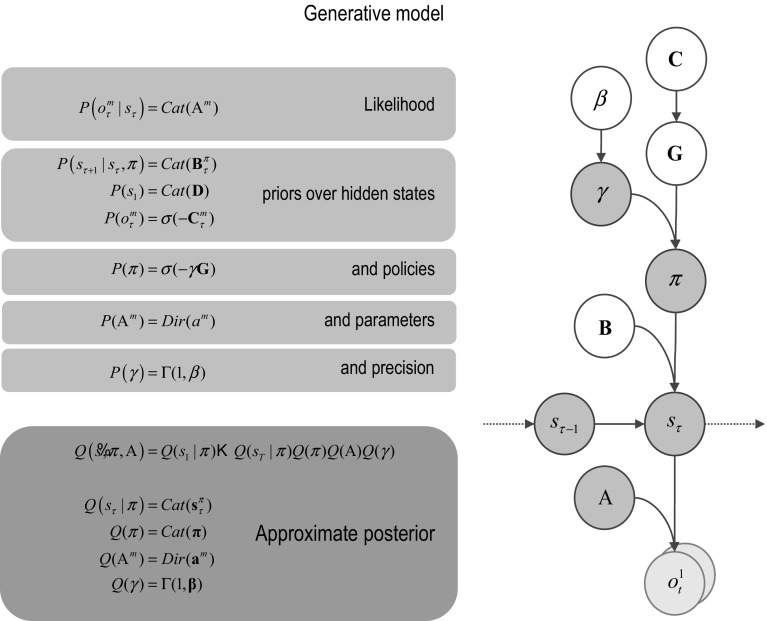
Fig. 1.

Generative model and (approximate) posterior. A generative model specifies the joint probability of outcomes or consequences and their (latent or hidden) causes. Usually, the model is expressed in terms of a likelihood (the probability of consequences given causes) and priors over causes. When a prior depends upon a random variable, it is called an empirical prior. Here, the likelihood is specified by matrices A whose components are the probability of an outcome under each hidden state. The empirical priors in this instance pertain to transitions among hidden states B that depend upon action, where actions are determined probabilistically in terms of policies (sequences of actions denoted by $\pi$). The key aspect of this generative model is that policies are more probable a priori if they minimise the (path integral of) expected free energy G. Bayesian model inversion refers to the inverse mapping from consequences to causes, i.e. estimating the hidden states and other variables that cause outcomes. In variational Bayesian inversion, one has to specify the form of an approximate posterior distribution, which is provided in the lower panel. This particular form uses a mean field approximation, in which posterior beliefs are approximated by the product of marginal distributions over unknown quantities. Here, a mean field approximation is applied both posterior beliefs at different points in time, policies, parameters and precision. Cat and Dir referred to categorical and Dirichlet distributions, respectively. See the main text and Table 2 for a detailed explanation of the variables. The insert shows a graphical representation of the dependencies implied by the equations on the right