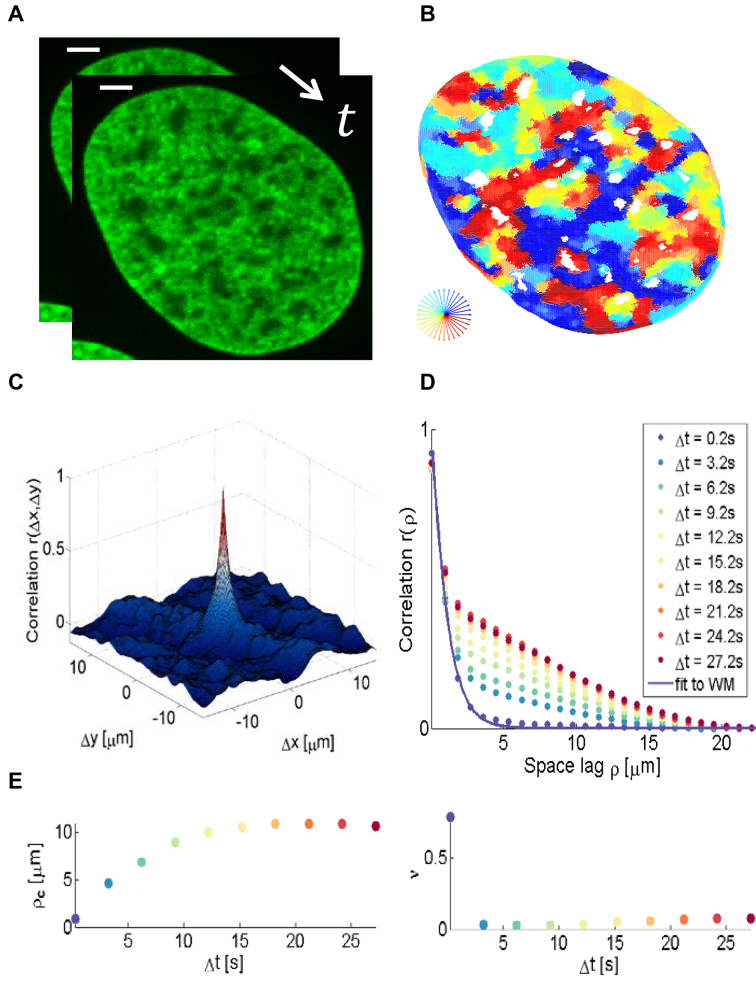
Figure 2.
Schematic representation of the correlation analysis. (A) Two microscopy images (U2OS cells expressing H2B-GFP) were acquired with temporal resolution 200 ms. Scale bar is 3 μm. (B) The flow field between the input images was estimated by the Horn–Schunck formulation and color-coded as indicated in the lower right. Pixels in nucleoli appear empty due to the lack of intensity information. (C) Correlation calculation in two dimensions. (D) Empirical correlation (example shown for direction) was calculated as a function of space lag and fitted to the WM correlation model. Flow fields were estimated at every accessible time lags within the image series and each of them was fitted (example time lags shown only). (E) Correlation length  and the smoothness parameter
  were derived from the regression and shown over the time lag. The parameters were averaged for each time interval over all accessible time points. Note that with increasing time interval, less time points are available and therefore, the standard deviation (not shown) increases.

