A Flow Procedure for Linearization of Genome Sequence Graphs

Abstract

Efforts to incorporate human genetic variation into the reference human genome have converged on the idea of a graph representation of genetic variation within a species, a genome sequence graph. A sequence graph represents a set of individual haploid reference genomes as paths in a single graph. When that set of reference genomes is sufficiently diverse, the sequence graph implicitly contains all frequent human genetic variations, including translocations, inversions, deletions, and insertions. In representing a set of genomes as a sequence graph, one encounters certain challenges. One of the most important is the problem of graph linearization, essential both for efficiency of storage and access, and for natural graph visualization and compatibility with other tools. The goal of graph linearization is to order nodes of the graph in such a way that operations such as access, traversal, and visualization are as efficient and effective as possible. A new algorithm for the linearization of sequence graphs, called the flow procedure (FP), is proposed in this article. Comparative experimental evaluation of the FP against other algorithms shows that it outperforms its rivals in the metrics most relevant to sequence graphs.

1. Motivation

The current human reference genome consists essentially of a single representative of each of the human chromosomes. In essence, an arbitrary person's genome is chosen to represent all of humanity. This leads to loss of information and bias. Efforts to incorporate human genetic variation into the reference human genome have converged on the idea of a graph representation of genetic variation within a species, a genome sequence graph (Paten et al., 2014).

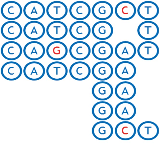
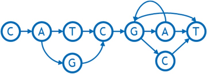
In its mathematically most simple form, each node of a sequence graph contains a single DNA base that occurs at an orthologous locus in one or more of the haploid genomes represented in the graph. Each arc represents an adjacency (chemically, a covalent bond) that occurs between consecutive instances of bases in those genomes. Excluding reversing joins (see Section 3.5), each arc is directed according to the default strand direction of the DNA sequence used to build the graph, connecting the 3′ side of the previous base (the tail of the edge) with the 5′ side of the next base (the head of the edge). At points where the individual genomes differ to the right (i.e., 3′, downstream) of an orthologous base, the node representing that base will have two or more outgoing arcs. For example, the aligned sequences shown in Figure 1 can be represented using the graph shown in Figure 2.

FIG. 1.

Alignment of CATCGCT, CAGCGAT, and CATCGAGAGAGCT DNA strands.

FIG. 2.

An example of a sequence graph reflecting SNP (T/G), tandem duplication GA -> GAGAGA, and deletion/SNP (A/C/-).

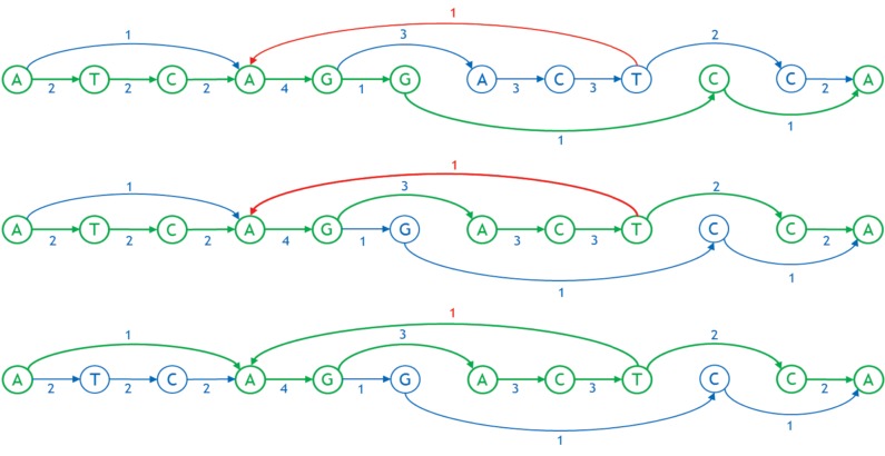
Representing a genome as a graph requires building a number of tools to work with it efficiently. In particular, one needs to linearize the graph, that is, order the nodes from left to right in a straight line. Linearization facilitates visual perception of a graph, allows software to index the nodes in a familiar manner, and imposes natural order of bases useful in storage, search, and analysis, for example, enabling traversal from left to right with minimum feedback runs. Figures 3 and 4 show examples of a linearized graph and individual genomes in it. Here, we have also added a new feature to the graphs in the form of arc weights. An arc weight is used to signify the importance of an arc in typical applications running on the graph. Normally, we set the arc weight to the number of times that the arc is traversed in the reference genomes used to build the graph, under the assumption that arcs used frequently in the reference genomes will also be used frequently in the applications of the sequence graph built from them. Some reference genomes may be weighted more than others.

FIG. 3.

An example of a linearized sequence graph with weighted arcs. The arc in red is directed from the right to the left and is called feedback arc.

FIG. 4.

Three individual genomes as paths in the linearized graph, shown in green. The first and second genomes are ATCAGGCA and ATCAGACTCA, respectively. The third genome is AAGACTAGACTCA wherein the arc between T and A is a feedback arc.

2. Problem Statement

A linearization of a sequence graph aims to make the total weight of all feedback arcs, called the weighted feedback (Fig. 3), small, along with the “width” (number of arcs) crossing any vertical line in the layout (called a “cut,” Fig. 5). Unnecessary feedback arcs make many types of genetic analysis more inefficient, as these typically proceed left to right on a conventional reference genome. An arc crossing a cut is considered to be part of an allele spanning that cut (Paten et al., 2017), so a graph with smaller cut width at a cut has fewer alleles at that cut. The mean of the cut width over all cuts in the graph is called the average cut width.

FIG. 5.

Examples of cuts and cut widths. Three cuts are shown with green vertical lines. Their widths are, from left to right, 3, 4, and 2, respectively.

In light of their importance for genetic analysis, we evaluate a linearization based on its average cut width and either the weighted feedback or the number of feedback arcs it contains.

Unfortunately, the problems of minimizing weighted feedback, and of minimizing the average cut width, are each separately difficult. The simpler problem of minimizing the number of feedback arcs is known in the literature as the feedback arc set problem, or FAS for short (Baharev et al., submitted). This is an NP-hard problem (Karp, 1972), but there are a number of various heuristic approaches to approximating a solution to it (Brandenburg and Hanauer, 2011). The problem of minimizing the average cut width (Gavril, 1977) is also known to be NP-hard. A good heuristic (Martí et al., 2013) is necessary for good results. In our case, starting our procedure with the “primary path” taken by the reference genome is a natural choice. This is the first time to our knowledge that a heuristic algorithm to minimize both metrics at the same time has been proposed.

3. Algorithm Description

We propose here a simple heuristic divide-and-conquer approach to linearly order the bases of a graph that tries to achieve either small weighted feedback (or small number of feedback arcs) and small average cut width. The key algorithmic tool is max-flow/min-cut in a directed graph (Cormen et al., 2009), so we call it the flow procedure (FP). Before applying the FP, the sequence graph is “groomed” as described at the end of this section.

3.1. First step: find the backbone

After grooming, the FP starts with a connected graph with directed arcs and a designated linear ordering of a subset of bases called the backbone. Arcs leading from the backbone to nodes not on the backbone are called out-arcs, and arcs directed into the backbone from nodes not on the backbone are called in-arcs. Grooming guarantees that the first base of the backbone has no in-arcs and the last has no out-arcs. Extra dummy bases are added at either end if necessary. Normally, the initial backbone is a biologically determined primary path of the graph, for example, from a selected haploid reference genome in the set of genomes used to build the graph, perhaps the existing haploid reference human genome. The FP creates a backbone using its internal heuristics if none is given a priori. In linearizing the sequence graph by creating a total ordering of the bases, the relative order of the bases in backbone will not change. The rest of the bases in the graph will be inserted either between bases of the backbone, before the backbone, or after the backbone. Thus, any feedback arcs already in the backbone ordering, called initial feedback arcs, will remain as feedback arcs in the final ordering.

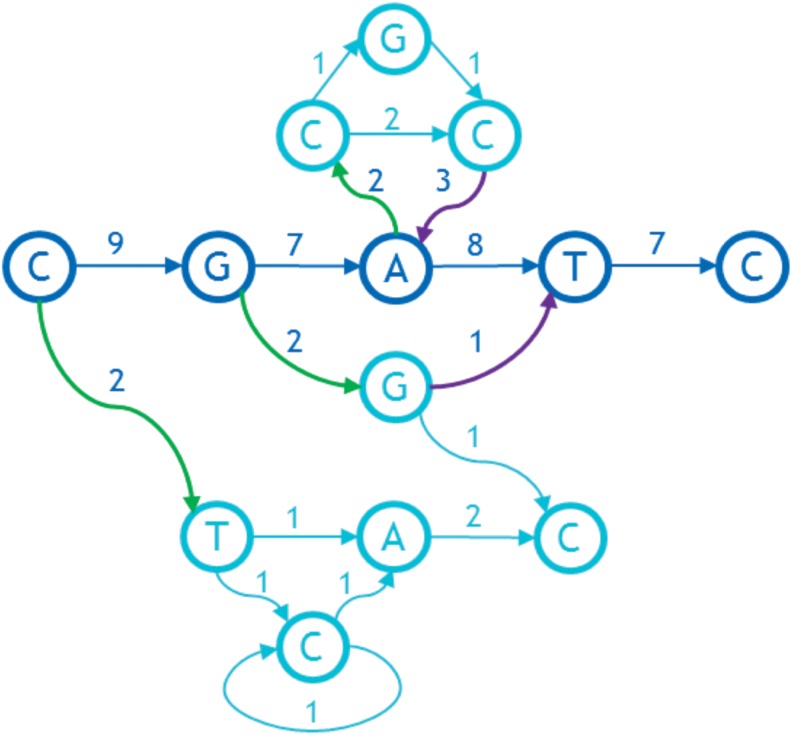
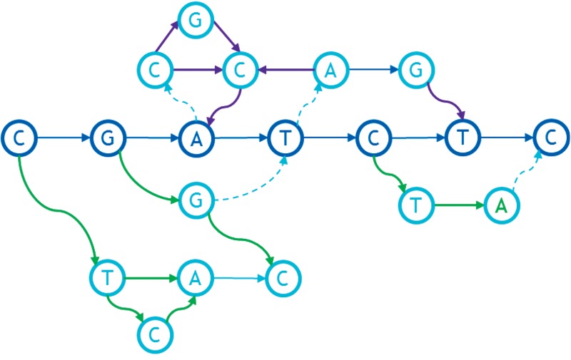
Consider the graph depictured in Figure 6. The backbone is the sequence CGATC horizontally across the middle (highlighted by dark blue). The three out-arcs of the backbone are shown with thick green arrows. The two in-arcs are shown with thick purple arrows. The weights are assumed to reflect usage, but we also assume that the usage statistics may be partial. Hence the weight coming into a base does not always match the weight coming out.

FIG. 6.

An initial directed graph with weights on the arcs.

3.2. Second step: add source and sink

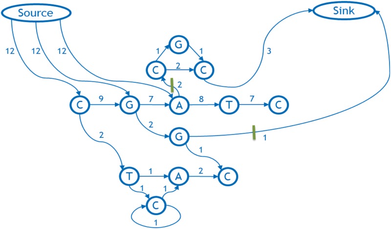
We set up a max-flow/min-cut network as follows. The nodes and arcs of the network are nodes and arcs of the graph. The capacity of the arc is its weight. In addition, there is a special source node and a special sink node. The network arcs for these are defined as follows: we let N be the maximum of the sum of the weights of the outgoing arcs for any node in the graph and we add an arc of capacity N + 1 from the source node to each base on the backbone that has an out-arc. Then each in-arc on the backbone is redirected to the sink node with no change in capacity.

3.3. Third step: determine the minimum cut and delete it

The maximum flow in our example is easily seen to be 3, and it maximizes the capacity of the two arcs that are cut by the green bars (Fig. 7). Therefore, these form a minimum cut. Since the capacities of the arcs connecting the source to the backbone are too high to be achieved by any flow, none of these are in the cut. Therefore, the cut must split the flow network into an out-component containing the source and its outgoing arcs, and an in-component containing the sink. Figure 7 shows the in-component consists of the uppermost nodes C, G, C, and the sink, and the out-component is the remainder.

FIG. 7.

The flow network corresponding to the above weighted graph and its designated backbone.

We remove the cut arcs from the graph. Essentially, in doing this we decide to give up worrying about these arcs and try to minimize the weighted feedback and average cut width as if they were not there. Since capacity equals weight, by choosing a minimum capacity cut, we ignore the arcs that cost us the least in weight.

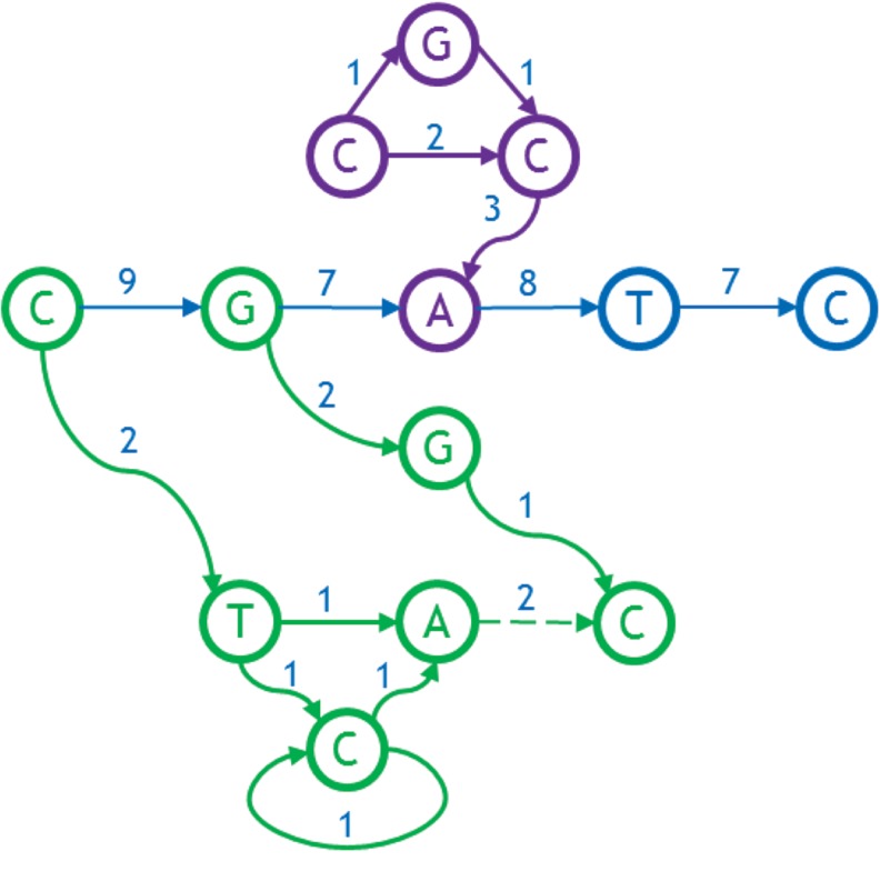
Excluding any initial feedback arcs on the backbone itself, we classify all bases not on the backbone into a sequence of outgrowths and ingrowths as follows. Starting at the last base on the backbone that has an out-arc, we define its outgrowth to be all bases reachable by a forward directed path from that base. Then we move backwards along the backbone, defining outgrowths consisting of all the bases reachable by a forward directed path from the base on the backbone with an out-arc that was not already included in previously defined outgrowths. We define ingrowths in a similar manner, moving forward from the start of the backbone and using backward-directed paths. Figure 8 shows ingrowth and outgrowths for the example under consideration. There are two outgrowths, the first from node G on the backbone (contains nodes G, G, and C), and the second from its predecessor, the first node on the backbone (labeled “C,” contains nodes C, T, C, and A). The dotted green arc is not a proper part of either outgrowth; it is discovered when exploring the outgrowth from C, and found to lead into the previous outgrowth found from G. The one ingrowth enters the node A of backbone and contains nodes C, G, C, and A, shown in purple.

FIG. 8.

Outgrowths (green) and ingrowths (purple) of the graph.

3.4. Fourth step: repeat procedure for ingrowth and outgrowth

Finally, we apply the entire procedure recursively to each outgrowth and ingrowth, using a heuristic that uses the backbone's base as the first base for an outgrowth or as the last base for an ingrowth, respectively. When the recursive call completes, the bases from it are inserted into the backbone of the calling procedure in the specified order immediately after an outgrowth or immediately preceding an ingrowth, respectively. The final ordering for the mentioned example is shown in Figure 9.

FIG. 9.

The final sorted graph with the bases totally ordered.

Normally the outgrowths and ingrowths together comprise the whole graph (see Section 7 for the case than they do not). However, if not, the entire procedure can just be repeated, each time using the linear order established from the previous cycle as a new backbone. Grooming a connected graph (see Section 3.5) assures that these repetitions will eventually reach every node in the graph.

It remains to specify a heuristic for determining the backbone when it is not explicitly given. When the first base of the backbone is given, we extend it into a path using a greedy algorithm: in each step, we add to the existing path the base with the highest forward directed arc weight that does not feedback to a node already in the backbone, breaking ties arbitrarily, and we do so until no more bases can be added. A complementary procedure is run in reverse if we are instead given the last base of the backbone.

3.5. Grooming

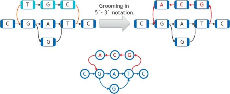
Finally, we explain the preprocessing step of grooming the graph. The base in each node in a sequence graph has two sides (3′ and 5′). The directed arcs we have been using are edges of the sequence graph that connect the 3′ side of one node to the 5′ side of another (possibly the same) node. The arcs are directed in the 3′ to 5′ side direction. There are also additional edges in a sequence graph that here we will refer to as reversing joins, which we have not discussed up until this point (see Paten et al. (2014) and Medvedev and Brudno (2009) for an introduction). A reversing join is an undirected edge connecting the 3′ sides of two nodes, or connecting the 5′ sides of two nodes. As a preprocessing step to the FP, and all other heuristic algorithms we examine for linearization of a directed graph, we first eliminate as many of the reversing joins as possible by replacing the graph with an equivalent graph that has fewer reversing joins. Then if there are still reversing joins left, we just ignore them. This way we are always working with graphs that only contain directed arcs. The process we use to minimize the number of reversing joins is called grooming (Fig. 10).

FIG. 10.

Grooming procedure. Reversing joins are shown in brown on the upper left. Bottom one shows the graph on the upper right as directed graph.

Grooming works as follows. A given connected component (a set of nodes such that one can travel between any two nodes in it along the standard arcs, in both directions, and using reversing joins) may fall apart if the reversing joins are removed. This indicates that some of the reversing joins were unnecessary. Let one connected component obtained after removing the reversing joins be called the primary component (shown in dark blue in Fig. 10), and the others be called the secondary components (shown in light blue in Fig. 10). We obtain an isomorphic graph that will have fewer components after removal of reversing joins by simply reverse-complementing the secondary components, that is, reverse-complementing every base in them and inverting the direction of the arcs between these secondary bases. The 3′ reversing joins connecting the secondary components to the main graph are replaced by directed arcs pointing into the secondary components, and the 5′ reversing joins are replaced by directed arcs back to the primary component. This has the effect of changing every 3′ side in a secondary component into a 5′ side, and vice versa. On the right side of Figure 10, nodes and arcs that were changed during grooming are shown in red. By repeating this procedure on any connected sequence graph, we eventually reach an isomorphic graph that has just one connected component even after removing the reversing joins.

Since we will not be reducing the number of reversing joins further, and being undirected, they cannot be considered feedback arcs; from here on, we will stop paying attention to the reversing joins and consider only graphs that are fully directed.

4. Analysis

4.1. Feedback arc set minimization

The FP's heuristic minimization of the feedback arc is based on the following property:

Claim: Each min-cut step of the algorithm removes the minimum weight set of arcs such that afterward there are no remaining paths that start on the backbone, leave the backbone, and then return to the backbone. We say the set of removed arcs have the “path-breaking” property.

Proof. First we will verify that the arcs removed in the min-cut step satisfy the path-breaking property. Suppose a path (p₀, p₁, …, p_n) remains such that p₀ and p_n (not necessarily distinct) are on the backbone and p₁, …, p_n–1 are outside the backbone. Note that (p₀, p₁) is an outgoing arc and (p_n–1, p_n) is an incoming arc. Thus, by construction, the flow network includes arcs (s, p₀) and (p_n–1, t), where s and t are the source and sink, respectively. Therefore (s, p₀, …, p_n–1, t) is a path in the flow network, which contradicts the fact that the removed arcs constitute an s–t cut.

To show that the cut has minimum weight, it suffices to show that any set of arcs satisfying the path-breaking property is an s–t cut. Minimality then follows from the fact that we removed the min-cut. Suppose we remove a set of arcs with the path-breaking property. Suppose there still exists a path (s, p₀, …, p_n–1, t) in the remaining graph. By construction, p_n–1 must be the head of an incoming arc (p_n–1, p_n) to the backbone that was not removed. Moreover, p₀ must be on the backbone. Therefore, path (p₀, p₁, …, p_n) is a path that starts on the backbone, leaves the backbone, and ends on the backbone, which is a contradiction to the assumed path-breaking property.   ■

Corollary: Every cycle in the graph is either (1) broken during the min-cut step of the algorithm or (2) entirely contained in the backbone of some recursive call.

Proof. Consider a cycle containing an arbitrary node x. In some recursive call, x will be in the backbone. If the cycle containing x was broken in some previous recursive call, the corollary is verified. Otherwise, the corollary follows from the previous claim.   ■

We can then define three sets of arcs based on a run of the FP:

• 1.F is the set of feedback arcs.
• 2.B is the set of feedback arcs whose head and tail were in the backbone of some recursive call.
• 3.C is the set of arcs that are removed by the min-cut steps.

It follows from the corollary that F ⊆ B ∪ C. This immediately yields a bound on the weight of the FAS.

where w(a) is the weight of an arc. Therefore, the FP can be seen as two alternating greedy heuristics (the backbone and the min-cut steps) that minimize an upper bound on the FAS. The backbone construction is greedy in that it always takes the remaining nonfeedback arc with the highest weight, leaving those with smaller arc weight. The min-cut is greedy in that it minimizes arc weight relative to a subset of all possible feedback arcs, namely those that fall on a path that visits, leaves, and then returns to the backbone.

4.2. Computational complexity

The max-flow/min-cut sorting algorithm already described can be broken into four steps:

• 1.Find the backbone (if it is not given).
• 2.Create the flow graph by adding the source and sink and connecting them to the graph.
• 3.Find the maximum flow and minimal cut and delete the minimal cut, using the Ford–Fulkerson algorithm.
• 4.Find the ingrowth and outgrowth and repeat steps 1 through 4 for them.

Let us consider the complexity of each step separately.

In the preparation step, we perform a greedy depth-first search to find the backbone if it is not given (in practice, we only find the backbone on recursive calls, as the whole graph's backbone is given). We do not visit any arc more than once, so the time complexity is O(|A|), where A is the number of arcs.

In creating the flow, we add two nodes to the graph (source and sink) and draw several arcs from the source to those nodes in the backbone that have an outgoing arc, and also reroute the arcs going into the backbone to the sink. We do not examine any arc more than once, so the time complexity is O(|A|).

The Ford–Fulkerson algorithm works in O(|A||max-flow|) (Ford and Fulkerson, 1962). In the worst case, |max-flow|∼O(|A|), in which case the time complexity becomes O(|A|²).

Every recursive call decreases the number of nodes in the graph, so the number of recursive calls is O(|V|), where V is the number of nodes.

These estimations are given in Table 1.

Table 1.

Complexity Estimation of the Flow Procedure Algorithm

Step	Complexity
1. Find the backbone	O(|A|)
2. Add source and sink, draw the arcs with required weights	|V|+| out-arcs and in-arcs | = O(|A|) assuming at least one arc per node
3. Determine the maximum flow and remove the arcs from the minimum cut	O(|A||max-flow|)
4. Repeat steps 1 through 4	Recursion depth ≤|V|

The final complexity estimate is thus O(|A||max-flow||recursion depth|).

The best-case complexity (if the max-flow is constant and there are a constant number of recursive calls) is O(|A|), again, assuming at least one arc per node. In the worst case, it is O(|A|²|V|), as the max-flow may be proportional to |A| and the recursion depth proportional to |V|.

The Ford–Fulkerson algorithm and the recursion contribute the most to the final algorithm's complexity. Depth of recursion is not a problem in practice. However, the maximum flow will often be approximately O(|A|) depending on how the flow is constructed: each variation increases it by creating a new path from the source to the sink. Because the flow becomes so large, the Ford–Fulkerson algorithm will work in quadratic time (O(|A|²)). Improvements to the algorithm that reduce the typical max-flow so that it is polylogarithmic in |A| would improve its speed.

5. Experimental Evaluation

5.1. Data modeling

1. The FP was tested on data that was artificially generated by taking a 37 kb piece of the GRCh38 assembly and adding artificial structural variations to it using the RSVSim (https://www.bioconductor.org/packages/release/bioc/html/RSVSim.html) from Bioconductor. This package lets one simulate any given set of structural variations to a reference, producing a modified FASTA file. The positions of the variations were distributed uniformly, while their lengths were fixed. After fixing a specified set of variations, a series of FASTA files were created and passed on to a vg (https://github.com/vgteam/vg) tool, which generated the graph using a multiple sequence graph alignment algorithm.

Four types of structural variation were simulated: insertions, deletions, duplications, and inversions. Tandem duplications were limited to one copy.

Two different test data sets, each consisting of a series of graphs, were generated in this way. The first was created to investigate the effect of the overall amount of variation on the number of feedback arcs and the cut width achievable by each algorithm. This data set consisted of graphs each having equal number of all four kinds of variations (i.e., there were as many insertions as there were deletions, inversions, and duplications), with only the total number of variations changing between graphs. The sizes of variations are given in Table 2. More details on data modeling could be found in the Section 7.

Table 2.

The Lengths of the Variations in the Testing Data

	Deletion	Insertion	Inversion	Duplication
Length	20	20	200	500

The second set of graphs was created to investigate the relationship between the relative frequencies of each type of variation and the number of feedback arcs and the cut width achievable by each algorithm (Haussler et al., 2017, tables 1–4).

The third data set was created to test the algorithm's time performance. The graphs in this data set were created from scratch and have structure similar to those graphs mentioned with doubling of the number of nodes from one to another.

5.2. Results and discussion

To comparatively analyze the quality and speed of our algorithm, we took Kahn's well-known topological sorting algorithm (Kahn, 1962), as well as Eades' (Eades et al., 1993) modified version thereof that guarantees a low number of feedback arcs while still working in linear time. We were not able to find a competitor for cut width minimization problem to measure against, because all the algorithms we have found are focused on exact solution of the problem, thus having high complexity (cubic and higher) and thus working only with graphs of 200 nodes or less. Note that neither Kahn's nor Eades' algorithm uses the backbone as a heuristic. All three algorithms were tested on the same data (see Section 4.1 for details on the modeling). Their outputs were compared on two metrics—the number of feedback arcs and the average cut width. Kahn's algorithm, Eades' algorithm, and FP are all implemented in the vg tool.

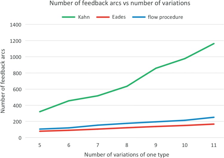
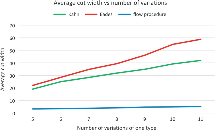
Figures 11 and 12 depict the main quantitative outputs of the three algorithms, Kahn, Eades, and the FP, for the first set of testing data. The same results for the second set are given in Haussler et al. (2017). From Figure 11 it is fairly obvious that in terms of the number of feedback arcs, the FP algorithm vastly outperforms Kahn's algorithm, doing only slightly worse than Eades' algorithm. The difference between FP and Eades algorithms is much smaller than between FP and Kahn algorithms. It is clear from Figure 12 that FP's average cut width is an order of magnitude lower than that of Eades or Kahn.

FIG. 11.

The relationship between the number of feedback arcs and variations.

FIG. 12.

The relationship between the ACW and number of variations.

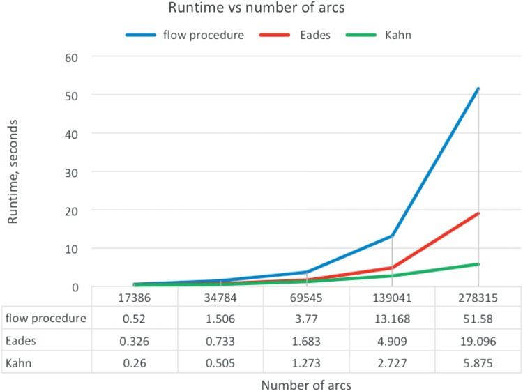
To use the FP algorithm in practice, one must estimate the time it takes the algorithm to run on large amounts of data. To use the algorithm on large graphs in practice, we would split the graph into pieces using a graph decomposition scheme as described in Paten et al. (2017). In practice, the time complexity of the FP is O(|A|²). In contrast, both Kahn's and Eades' algorithms have complexity O(|A|+|V|), since they do not pass any node more than twice. The relationship between the number of nodes in the graph and the algorithms' runtimes on our test data is shown in Figure 13.

FIG. 13.

The relationship between the runtime and the number of arcs in the graph.

The relationship matches the one predicted theoretically. It shows that despite quadratic complexity estimation, it is clearly seen from Figure 13 that the algorithm can be used on big graphs.

In addition to these tests on synthetic data, the algorithms were tested on a graph created from the human major histocompatability complex (MHC) region of chromosome 6 with 251,297 nodes. FP running time was about 40 minutes.

6. Conclusion

We have proposed a new sequence graph linearization algorithm that outperforms standard methods on the criteria that are important for storing, traversing, analyzing, and visualizing genome sequence graphs. The quantitative results thus obtained suggest that this algorithm will prove useful in genome exploration. Earlier work on sequence graph linearization (Nguyen et al., 2015) focused on minimizing feedback arcs, here we additionally introduce cut-width as an important measure of a linearization that effectively measures contiguity between elements that are connected. Future effort to lower the computational complexity of the algorithm using graph decomposition (Paten et al., 2017) could allow us to apply a modified form of the presented algorithm to complete human scale sequence graphs of hundreds of millions of nodes.

7. Appendix

7.1. Some details of the FP algorithm

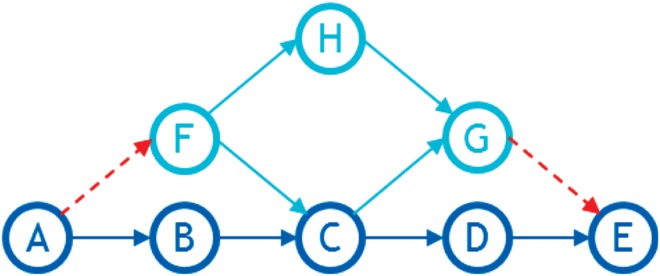
We pointed out in the algorithm description that sometimes not all of the graph's nodes end up in the final list, and so we need to rerun the procedure with the graph's sorted part as the backbone. Figure 1 demonstrates an example of such a situation.

Here, ABCDE is the backbone (shown in dark blue), arcs AF and GE are in the min-cut and hence deleted in the first run (Fig. 14). CG is the ingrowth and FC is the outgrowth. Node H is in neither the ingrowth nor in the outgrowth and so does not end up in the list on the first run of the procedure. On the rerun, however, the backbone will be ABFCGDE and so H will fall into F's outgrowth.

FIG. 14.

An example of a graph that requires a rerun.

Also noteworthy is the order in which we find the ingrowth and outgrowth. First, we traverse the backbone from end to start, finding the outgrowth for each node, then we traverse it from start to end, finding the ingrowth. We include in the ingrowth and outgrowth only those nodes that did not end up in any of the previous outgrowth or ingrowth (Fig. 2).

7.2. Step-by-step algorithm run

Let us start from the moment when we have already found and removed the minimum cut (Fig. 15). We go from the beginning to the end over the backbone (CGATC) and find the ingrowth CCGA (upper three nodes and A from the backbone). For this ingrowth, we run the entire FP recursively. Looking for the backbone, we start from A and search for incoming max weight arcs. We get CCA, then run the min-cut search and remove the CG arc. Then we recursively go to the CCA backbone from the beginning to the end; we are looking for the ingrowth. We find GC. For it, we run the procedure, which arranges these two nodes in the obvious way. We insert the result into the backbone CCA with the G before the second C (the one that had the in-arc). Thus, we get CGCA. All nodes of this part are sorted, so the recursion is finished and we insert the resulting ingrowth into the backbone of the source graph. Inserting to the backbone we get CGCGCATC. There are no other ingrowths, so we turn to search for outgrowths. We go from the end to the beginning. We find the GGC outgrowth. It includes three consecutive nodes, so the recursive procedure for it throws out a natural GGC order. We insert to the backbone and get CGGCCGCATC. Then we look for the next outgrowth. We find the CTCA starting from the first node of the backbone. For it, we run the procedure recursively. It finds the backbone CTA, then removes the min-cut, finds the ingrowth CA, and inserts its C before the A: CTCA. There are no other ingrowth or outgrowths, so this part of the algorithm is finished and we insert nodes to the original backbone, finally getting CTCAGGCCGCATC.

FIG. 15.

An example of the ingrowths and outgrowths for a graph.

7.3. Test data set modeling

To simulate the test data, we used the RSVSim package (version 1.14.0) from the Bioconductor software (Release 3.4). As a reference genome, we took BSgenome.Hsapiens.UCSC.hg38 (version 1.4.1), alternative branch chr13_KI270842v1_alt, which is 37287 nucleotides long. Using the simulateSV command of the RSVSim package, we modeled genome fragments of 10 individuals with a given set of variations. Resulting FASTA files were submitted to the entry of the msga command of the vg utility (https://github.com/vgteam/vg). As a result, we got a sequence graph (*.gfa format). This graph is an input to the commands vg sort-f (Eades) and vg sort (FP) of the vg utility (https://github.com/vgteam/vg). Finally, we got text files with graph nodes ordered by linearization using the Kahn, Eades, and FP algorithms, respectively. To analyze the algorithm, we created the original software to get the number of feedback arcs and the cut width in the mentioned sorts. To reduce the variance of estimates, we repeated the procedure 20 times for each set of variations and averaged the results.

We created variation sets as follows. In the modeled genome fragments, we added five variation types: insertions, deletions, duplications, inversions, and translocations. The positions of all variations were uniformly distributed over the simulation section of the genome. Twenty percent of the insertions were duplicating sections of the DNA. Translocations were modeled using the shoulder exchange mechanism. The lengths of insertions and deletions were 20 nucleotides, the length of inversion was 200 nucleotides, and the length of duplications was 500. The number of variations of each type was equal to 5 in the first set, 6 in the second, 7 in the third, and so on up to 11 in the latest set of variations. Haussler et al. (2017) provide a dependence of the number of feedback arcs and cut widths of number of variations of the same type. For this study, the number of variations of all types, except the examined, was fixed at level 7, and the number of investigated variations was changing according to the following list: 7, 9, 11, 13, 15, 17, 19, 21, 23, 25, 27, 29, and 31.

Acknowledgments

The authors thank Erik Garrison and Glenn Hickey for helpful conversations. This work was supported by the National Human Genome Research Institute of the National Institutes of Health under Award Number 5U54HG007990 and grants from the W.M. Keck Foundation and the Simons Foundation. The content is solely the responsibility of the authors and does not necessarily represent the official views of the National Institutes of Health.

Author Disclosure Statement

No competing financial interests exist.

References

- Baharev A., Schichl H., Neumaer A., et al. . submitted. An exact method for the minimum feedback arc set problem. Available at: www.mat.univie.ac.at/∼herman/fwf-P27891-N32/minimum_feedback_arc_set.pdf Last viewed: Jan. 2017
- Brandenburg F., and Hanauer K. 2011. Sorting heuristics for the feedback arc set problem. Technical Report MIP-1104. Department of Informatics and Mathematics, University of Passau, Germany [Google Scholar]
- Cormen T., Leiserson C., Rivest R., et al. . 2009. Introduction to Algorithms. MIT Press: Cambridge, Massachusetts [Google Scholar]
- Eades P., Lin X., and Smyth W. 1993. A fast and effective heuristic for the feedback arc set problem. Inf. Process. Lett. 47, 319–323 [Google Scholar]
- Ford L.R., Jr., and Fulkerson D.R. 1962. Flows in Networks. Princeton University Press: New Jersey [Google Scholar]
- Gavril F. 1977. Some NP-complete problems on graphs, 91–95. Proceedings of the 11th conference on information Sciences and Systems [Google Scholar]
- Haussler D., Smuga-Otto M., Paten B., et al. . 2017. A flow procedure for the linearization of genome sequence graphs. biorxiv. https://doi.org/10.1101/101501 [DOI] [PMC free article] [PubMed]
- Kahn A. 1962. Topological sorting of large networks. Commun. ACM. 5, 558–562 [Google Scholar]
- Karp R.M. 1972. Reducibility among combinatorial problems, 85–103. In Miller R.E., Thatcher J.W., Bohlinger J.D., eds. Complexity of Computer Computations. The IBM Research Symposia Series, Springer: Boston, Massachusetts [Google Scholar]
- Martí R., Pantrigo J., Duarte A., et al. . 2013. Branch and bound for the cutwidth minimization problem. Comput. Oper. Res. 40, 137–149 [Google Scholar]
- Medvedev P., and Brudno M. 2009. Maximum likelihood genome assembly. J. Comput. Biol. 16, 1101–1116 [DOI] [PMC free article] [PubMed] [Google Scholar]
- Nguyen N., Hickey G., Zerbino D., et al. . 2015. Building a pan-genome reference for a population. J. Comput. Biol. 22, 387–401 [DOI] [PMC free article] [PubMed] [Google Scholar]
- Paten B., Novak A., and Haussler D. 2014. Mapping to a reference genome structure. eprint arXiv:1404.5010 [Google Scholar]
- Paten B., Novak A.M., Garrison E., et al. . 2017. Superbubbles, ultrabubbles and cacti, 173–189. International Conference on Research in Computational Molecular Biology (RECOMB 2017), Hong Kong, China: [DOI] [PMC free article] [PubMed] [Google Scholar]