Abstract
Dynamic Causal Modelling (DCM) is an advanced biophysical model which explicitly describes the entire process from experimental stimuli to functional magnetic resonance imaging (fMRI) signals via neural activity and cerebral hemodynamics. To conduct a DCM study, one needs to represent the experimental stimuli as a compact vector-valued function of time, which is hard in complex tasks such as book reading and natural movie watching. Deep learning provides the state-of-the-art signal representation solution, encoding complex signals into compact dense vectors while preserving the essence of the original signals. There is growing interest in using Recurrent Neural Networks (RNNs), a major family of deep learning techniques, in fMRI modeling. However, the generic RNNs used in existing studies work as black boxes, making the interpretation of results in a neuroscience context difficult and obscure.
In this paper, we propose a new biophysically interpretable RNN built on DCM, DCM-RNN. We generalize the vanilla RNN and show that DCM can be cast faithfully as a special form of the generalized RNN. DCM-RNN uses back propagation for parameter estimation. We believe DCM-RNN is a promising tool for neuroscience. It can fit seamlessly into classical DCM studies. We demonstrate face validity of DCM-RNN in two principal applications of DCM: causal brain architecture hypotheses testing and effective connectivity estimation. We also demonstrate construct validity of DCM-RNN in an attention-visual experiment. Moreover, DCM-RNN enables end-to-end training of DCM and representation learning deep neural networks, extending DCM studies to complex tasks.
Keywords: Recurrent Neural Network, Dynamic Causal Modeling, functional magnetic resonance imaging, causal architecture, effective connectivity
1 Introduction
Dynamic Causal Modelling (DCM) (Friston et al., 2003) is a nonlinear generative model, the only one that models explicitly the entire process from stimulus to functional magnetic resonance imaging (fMRI) blood oxygen level dependent (BOLD) signal via neural activity and cerebral hemodynamics. It is thus considered by many to be the most biologically plausible as well as the most technically advanced fMRI modeling method (Smith, 2012)(Smith et al., 2013). A causal brain architecture, defined in terms of effective connectivity, describes how neural activity in distributed brain regions influence each other - and how input stimuli perturb neuronal dynamics. DCM is classically used to test hypotheses of causal brain architectures and estimate associated brain effective connectivity. Various approaches have been proposed for DCM parameter inference, such as Expectation Maximization (EM) Gauss-Newton search (Friston, 2002), variational Bayes (Friston et al., 2010, 2007, 2008; K. J. Friston, 2008), Kalman filtering methods (Daunizeau et al., 2009)(Havlicek et al., 2011), and Markov Chain Monte Carlo (MCMC) methods (Chumbley et al., 2007)(Aponte et al., 2016). DCM has enjoyed a rapid popularity uptake over the past decade (Friston, 2011). To conduct a DCM study, one needs to represent the experimental stimuli as a vector valued function of time. In simple paradigms, one entry in the stimulus vector can be a box train function to represent the on-off of an experimental condition or a continuously valued function to represent the intensity of an experimental condition. However, in complex paradigms such as book reading and natural movie watching, manually designing a compact vector representation of the complex stimuli, preserving the high level semantic meaning of the original signal, is very hard. Deep neural networks (DNNs) have been shown useful in representation learning, leading to state-of-the-art performance in various applications (Bengio et al., 2013). It is tempting to explore its use in DCM modeling.
Deep learning, which has shown considerable potential in the last decade as a powerful tool for data analysis, can help explore new possibilities of understanding of brain behavior (Gonzalez et al., 2017). As a major family of deep learning techniques, Recurrent Neural Network (RNN) is particularly suitable for temporal signals, e.g. fMRI, because it models temporal correlation among data explicitly with its recurrent structure. Recently, there is growing interest in using RNN to model fMRI signal (Gonzalez et al., 2017)(Barak, 2017). Specifically, Güçlü et al. (Güçlü and van Gerven, 2016) used RNNs to predict brain activity in response to natural movies to elucidate how complex visual and audio sensory information was represented in the brain. Qian et al. (Qian et al., 2016) trained a RNN to predict coming words in a book and were able to predict fMRI activity in reading subjects using hidden states in the RNN through linear mapping, suggesting a relationship between the RNN architecture and the cognitive process of reading. In addition, Sussillo et al. (Sussillo et al., 2015) trained RNNs to reproduce muscle activity in monkeys to explore the hypothesis that motor cortex reflects dynamics appropriate for generating temporally patterned outgoing commands. However, a major criticism of the use of generic RNNs in understanding biological processes is the lack of biophysical meaning.
Here, we harness the strengths of DCM to leverage its biophysical interpretability and extend this advantage to the nascent area of study applying RNNs to model fMRI signal. We introduce DCM-RNN, a biophysically interpretable RNN. We cast DCM into a novel generalized recurrent neural network (G-RNN) without any compromise of biophysical significance. The hidden states of DCM-RNN are neural activity, blood flow, blood volume, and deoxyhemoglobin content and its parameters are quantities such as effective connectivity, oxygen extraction fraction at rest, and vessel stiffness. DCM-RNN finds the maximum a posteriori (MAP) estimations of its parameters with back propagation. We believe DCM-RNN is a versatile tool. It can fit seamlessly into the classic DCM study pipeline for model evidence calculation and effective connectivity estimation. Moreover, its RNN architecture allows a straightforward combination of DCM-RNN with other (representation learning) DNNs and enables end-to-end training. The optimal representation is task dependent because the learnt representation should preserve any information related to the task and remove any nuisances variance (Achille and Soatto, 2018). End-to-end training ensures that the representation and DCM-RNN are optimized jointly.
In the remainder of this paper, we first provide backgrounds on DCM and RNN in Sec. 2, including model evidence and free energy bound. In Sec. 3, we explicate the development of DCM-RNN: the conversion of DCM into DCM-RNN, parameter estimation in DCM-RNN, and important implementation details of DCM-RNN on a deep learning platform. In Sec. 4, we show effective connectivity estimation and model selection with DCM-RNN in classical simple-stimulus scenarios. The results are compared with DCM. Finally, Sec. 5 presents possible extensions of DCM-RNN to accommodate other variants of DCM. Sec. 6 summarizes the main contribution of the paper. DCM-RNN studies with complex stimuli and DNN learnt representation will be explored in future work.
2 Backgrounds
2.1 Dynamic causal modeling
DCM can be expressed compactly as
| (1) |
| (2) |
where is the experimental or exogenous stimuli, the inputs to DCM. is the neural activity and is the modeled blood-oxygen-level dependent (BOLD) signal. is random fluctuation in the neural activity space which may be Wiener process (Daunizeau et al., 2009)(Havlicek et al., 2011), or analytic motion in the generalized coordinates (Friston et al., 2008)(K. J. Friston, 2008)(Friston et al., 2010), or absent (Friston et al., 2003). is observation noise which may be Gaussian or analytic motion in generalized coordinates (Friston et al., 2008)(K. J. Friston, 2008)(Friston et al., 2010). u, x, y, w, z are continuous-time functions of time t. θ is the whole set of DCM parameters, encoding the causal brain architecture, and typically treated as constant. The superscript M indicates the number of stimuli. Each stimulus is indexed as um, m ∈ {1, 2, … Nb}, is a scalar function, an abstract descriptions of the neural activity in the n-th brain region. yn (t), n ∈ {1, 2, … Nb} is a scalar function which is a summary of the fMRI signals in the n-th brain region, often obtained by averaging over all voxels in the region. As per convention, temporal derivative is denoted by a dot above a variable. f models the evolution of the neural activity and will be referred to as neural evolution function in this manuscript.g maps the neural activity to modeled fMRI and will be referred to as the hemodynamic function in this manuscript.
Fig. 1 shows an overview of the original DCM proposed in (Friston et al., 2003). In the original DCM, w is absent, and the neural evolution function takes a bilinear form as the majority of DCMs do:
| (3) |
where , for are parameters to be estimated, referred to as the effective connectivity (Friston, 2011). A indicates how the neural activity in one region influences those in other regions. Bm indicates how the m-th input stimulus alters the connectivity between regions. C indicates the impact of the input stimuli on the regional activities.
Fig. 1.
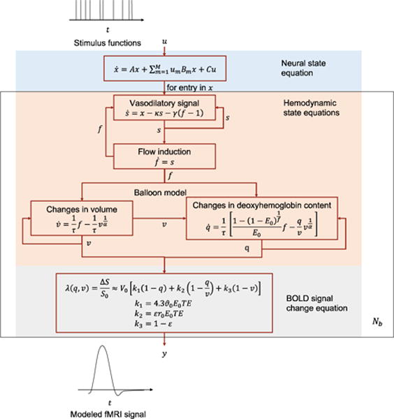
An overview of the original DCM.
While the neural activity is coupled between brain regions, the hemodynamics of one region does not depend on other regions, given the neural activity in that region. We drop the region index n of the DCM states and parameters in Eq. (4)–(9) for simplicity and clarity. First, x evokes vasodilatory signal s, which modulates the blood inflow f to a brain region (Friston et al., 2000)
| (4) |
| (5) |
where κ is a constant of signal decay and γ is a constant of feedback regulation. The blood volume change in a brain region is determined by blood inflow and outflow(Buxton et al., 1998)
| (6) |
where v is the volume of blood in a brain region, fout is blood outflow, the volume of blood leaving the brain region, and τ is mean transit time of blood. The blood outflow is a function of the blood volume based on the balloon model for vasculature (Grubb RL Jr, Raichle ME, Eichling JO, 1974):
| (7) |
where α is vessel stiffness. Under the assumption that oxygen extraction is tightly coupled to blood flow (Buxton et al., 1998)
| (8) |
where q is deoxyhemoglobin content, E0 is the oxygen extraction fraction at rest. A generalized BOLD signal model is proposed in (Stephan et al., 2007), which states that the modeled BOLD signal is a function of v and q
| (9) |
k1 = 4.3ϑ0E0TE
k2 = εr0E0TE
k3 = 1 − ε
where v0 is the resting venous blood volume fraction, ϑ0 is the frequency offset at the outer surface of the magnetized vessel for fully deoxygenated blood, E0 is the oxygen extraction fraction at rest, ΤE is the Echo Time, r0 is the slope of the relation between the intravascular relaxation rate and oxygen saturation, and ε is the ratio of intra- and extravascular signal.
As a summary, DCM describes each brain region with five state values {x, s, f, v, q}. Only the neural state x has interactions among regions. Hemodynamic states {s, f, v, q} work on each region separately and are only dependent on the neural state x in the same region. The whole model parameter set θ = {θC, θh, θλ} includes connectivity parameters θC, hemodynamic parameters θh and hyper parameters θλ as in Eq. (10) to Eq. (12).
| (10) |
| (11) |
| (12) |
Note that we drop the region index n of the DCM states and parameters in Eq. (4)–(9). Each element in θh is a Nb-dimensional vector, including the corresponding parameters in all brain regions (e.g. ). In the original DCM, the hyper parameters θλ are used to model the covariance of the Gaussian observation noise z.
In a particular study or a particular DCM implementation, θ can be reduced to one of its subset, by setting other parameters to known values based on prior studies. The same hemodynamic parameters for different brain regions can be constrained to have the same values. Table 1 summarizes the variables in DCM and their characteristics. θC is typically unknown before conducting an inference experiment while one may have hypothesis about the support of the matrices. An entry in a matrix in θC is allowed to deviate from non-zero in parameter estimation only if it is supported; otherwise, it is kept zero.
Table 1.
Notations in DCM and their characteristics.
| Meaning | Note | |
|---|---|---|
| u | Input stimulus | experimentally given |
| X | Neural state: Neural activation | Unknown hidden state |
| w | Random fluctuation in neural space | Unknown |
| s | Hemodynamic state: vasodilatory signal | Unknown hidden state |
| f | Hemodynamic state: Blood flow induction | Unknown hidden state |
| v | Hemodynamic state: Blood volume | Unknown hidden state |
| q | Hemodynamic state: Deoxyhemoglobin content | Unknown hidden state |
| y | fMRI signal | measured |
| z | Observation noise | Unknown |
| A | Connection parameter | weak prior, tunable |
| B | Connection parameter | weak prior, tunable |
| C | Connection parameter | weak prior, tunable |
| κ | Constant of signal decay | With prior, tunable |
| γ | Constant of feedback regulation | With prior, tunable |
| τ | Mean transit time of blood | With prior, tunable |
| E0 | Oxygen extraction fraction at rest | With prior, tunable |
| α | Vessel stiffness | With prior, tunable |
| V0 | Resting venous blood volume fraction | With prior, tunable |
| θ0 | Frequency offset at the outer surface of the magnetized vessel for fully deoxygenated blood | With prior, tunable |
| r0 | Slope of the relation between the intravascular relaxation rate and oxygen saturation | With prior, tunable |
| ε | Ratio of intra- and extravascular signal | With prior, tunable |
| λ | Noise related hyper parameters | May be estimated in advance, tunable |
| TE | Echo Time | experimentally given |
| M | Number of stimuli | experimentally given |
| t | Scan time | experimentally given |
| Nb | Number of brain regions | experimentally given |
• With prior: mean and/or variance can be found from previous neuroscience studies
• Weak prior: only support may be hypothesized, mean and variance are not biophysically informative
2.2 Model evidence and free energy
One of the principal uses of DCM is to evaluate the model evidence for different hypotheses given data and use Bayesian model comparison to adjudicate between hypotheses. A hypothesis is a particular combination of {f, g, w, z} and prior distributions associated with the combination. For example, one can use different forms of f to have nonlinear neural evolution function DCM (Stephan et al., 2008) and multiple neural states DCM (Marreiros et al., 2008). One can have deterministic DCM (Friston et al., 2003) by removing w in the neural evolution function and stochastic DCM (Friston et al., 2008)(K. J. Friston, 2008)(Friston et al., 2010) in the present of w. One can also control the causal architecture by setting the supports of θC, which is equivalent to set the non-supported connectivity with 0 mean and 0 variance in prior. Model evidence ln p(y|m) is the logarithm of the probability of seeing the fMRI data y given a model m. Here y is the fMRI signals from all brain regions and all time. The model evidence is usually not tractable and DCM resorts to variational Bayes for an approximation under the Laplace approximation. In variational Bayes, the model evidence can be expressed as
| (13) |
where F is the free energy, D is the Kullback-Leibler (KL) divergence, E is the expected energy, and H is the entropy of q. q is the variational distribution used to approximate the hard-to-track p(θ|y, m). Since D is always non-negative, F forms a lower bound of the model evidence, which is known as an evidence lower bound (ELBO) in machine learning. In DCM, q takes Gaussian form q(θ) = N(μq, Σq) and consequently the entropy of q is
| (14) |
where Np is the number of parameters. The Laplace approximation expands ln p(θ, y|m) as a Taylor series of θ up to the second order term at a mode of θ. Denote the optimal q, . The expected energy E can be approximated as (Friston et al., 2007)
| (15) |
The Laplace approximation is equivalent to assume that p(θ, y|m) is Gaussian with respect to θ and the majority probability mass of θ is concentrated at the mode . Substitute Eq. (14)(15) into Eq. (13),
| (16) |
Take derivative of the right-hand sides of (16) and set it to 0, one obtains the optimal covariance:
| (17) |
Substitute Eq. (17) into Eq. (16)
| (18) |
If . The free energy bound is tight and thus can be used to approximate the model evidence,
| (19) |
In DCM, q* is found by maximizing the free energy bound F. μq and Σq are optimized iteratively and Σq provides the curvature information used in the μq updating:
until converge:
| (20) |
| (21) |
end
Newton’s method is used to update and iteratively in the μq step. In the conventional way of using the Laplace approximation, is found first by any optimization solver according to Eq. (20) and is calculated post hoc (Friston et al., 2007).
2.3 Recurrent Neural Network
Different from other deep learning neural networks, which assume samples are independent, RNN respects the fact that samples are highly correlated in many applications, such as frames in video and words in a sentence. RNN models the correlation explicitly using the recurrent structure and thus is particularly suitable for sequence signal, such as fMRI. RNN has two typical graphic representations as shown in Fig. 2. Fig. 2(a) is a compact representation where the dashed line means the arrow points from current time point to the next. Fig. 2(b) is the unfolded RNN through time. In this representation, there is no explicit recurrent unit, but it is essential to see that an input of the system has an influence on current and future outputs.
Fig. 2.
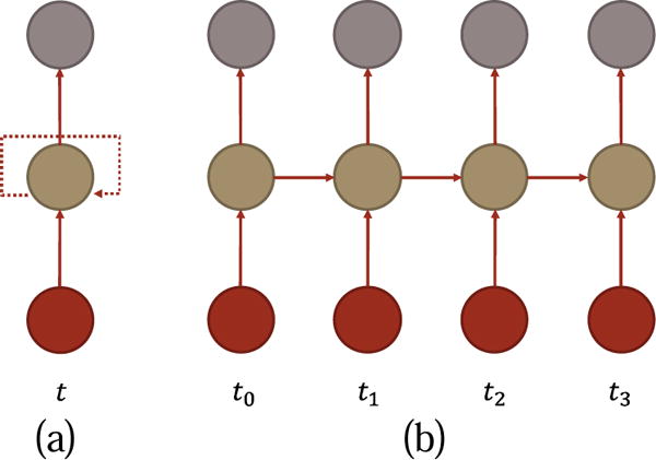
Typical graphic representations of a RNN. (a) compact. The dashed line indicates the recurrent structure (b)unfolded along time. I, H, and O stand for input, hidden state, and output respectively.
Multiple computational models can reside on the graphic structure in Fig. 2. The classic RNN (Zachary C. Lipton, 2015) models the relationship between its input and output as
| (22) |
| (23) |
where x is the input, h is the hidden state, and yt is the output. W and b are weighting matrix and bias, the tunable parameters. Subscript t indicates time and superscripts are used to differentiate parameters. fh and fy are simple nonlinear functions. For example, fh can be sigmoid or rectified linear unit, and fy is often softmax for classification and density approximation problem. A well-known shortcoming of the classic RNN is that it cannot capture long term correlation. Long short-term memory (LSTM) (Hochreiter et al., 1997) and Gated Recurrent Unit (GRU) (Cho et al., 2014) attenuate the problem by using gate units to lock information in the memory cells. RNNs have many other enhancements. Bidirectional recurrent neural network (Schuster and Paliwal, 1997) explores correlation from both forward and backward directions of a sequential signal. LSTM with attention (Dzmitry Bahdana et al., 2015) imposes an explicit mechanism of highlighting crucial information. LSTM with external memory (Graves et al., 2014) provides RNN with even more power of capturing long term dependency in the data. LSTM with Generative Adversarial Net (Dzmitry Bahdana et al., 2015) enables LSTM to generate realistic signals with the help of a discriminative model.
RNNs commonly use Backpropagation Through Time (BPTT) (Werbos, 1990)(Zachary C. Lipton, 2015) for training. BPTT treats RNN in the unfolded fashion. In this view, RNN is no longer a recurrent network, but a deep feedforward neural network. The error at one time point can be propagated back until the first time point. After propagating back all the errors, parameters are updated simultaneously, where the gradient for a particular parameter is the sum of partial gradients of errors from all the time points with respect to the parameter. A practical modification of the naïve BPTT is Truncated Backpropagation Through Time (TBPTT) (Williams and Zipser, 1989) which fixes the maximum number of time steps any error is allowed to propagate back. It alleviates the gradient vanishing/exploding problem suffered by BPTT.
3 Method
3.1 Convert DCM into DCM-RNN
We start the conversion from a generalization of the classic RNN by adding more nonlinearity into the classic RNN
| (24) |
| (25) |
ϕh and ϕy are the added nonlinear functions, which are parameterized by ξh and ξy. This generalization greatly extends the flexibility of RNN and makes the resulting G-RNN capable of accommodating the complexity of DCM.
Practically acquired fMRI data are discrete signals, which requires DCM to be discretized. In classic DCM, the discretization is based on a local linearization with matrix exponential (Ozaki, 1992). We use simple Euler’s method:
| (26) |
where Δt is the time interval between adjacent time points. This approximation can be arbitrarily accurate as long as Δt is small enough. Taking as an example. Substituting Eq. (26) into the neural evolution equation, Eq. (3) becomes
| (27) |
It can be organized and rewritten in the form of G-RNN
| (28) |
where B = [B1, B2, …, BM] is a concatenation of the Bm matrices and
| (29) |
where ⊗ is Kronecker product (Cichocki et al., 2015) defined as
| (30) |
Eq. (28) can be implemented as a part of a G-RNN shown in Fig. 3. Applying similar approximation to the hemodynamic equations, Eq. (4)–(8) become
| (31) |
| (32) |
| (33) |
| (34) |
Fig. 3.
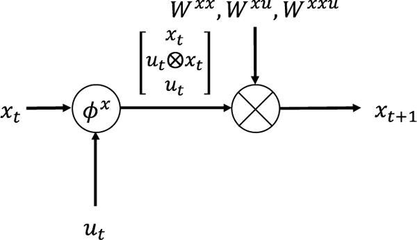
Neural evolution equation as a piece of G-RNN.
Grouping hemodynamic states {s, f, v, q} into a vector and some of their functions into one nonlinear function leads to Eq. (37), where
| (35) |
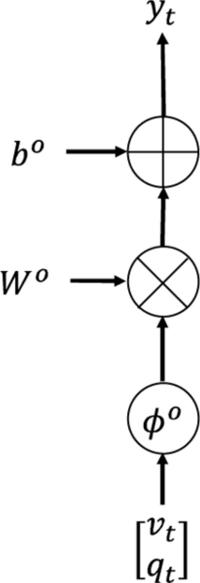
Eq. (26) can be implemented as a part of a G-RNN shown in Fig. 4. The fMRI output equation Eq. (9) is not a differential equation and can be directly rewritten without approximation to Eq. (38) where
| (36) |
Fig. 4.
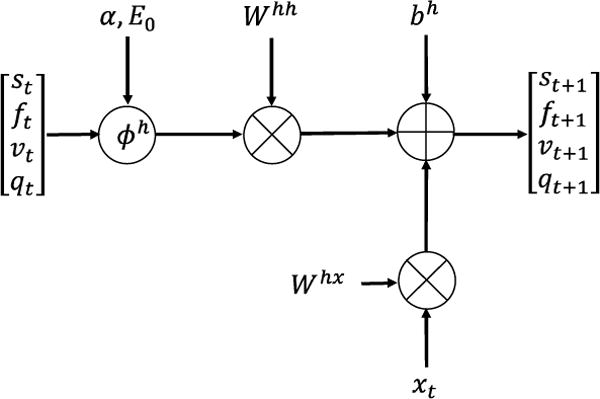
Hemodynamic equations as a piece of G-RNN.
Fig. 5 visualizes it as a piece of G-RNN.
Fig. 5.
Output equation as a piece of G-RNN.
Assembling all the pieces together, one obtains the final DCM in the G-RNN framework, shown in Fig. 6. In Fig. 6, variables are marked with both indicators in DCM and indicators in DCM-RNN to stress their relationship. The large rectangle over the hemodynamic and the output layer means the content inside the rectangle is repeated for each brain region. Repetition time is Nb as shown in the right bottom corner of the rectangle. Variables inside the rectangle are specific to each brain region.
| (37) |
| (38) |
Fig. 6.
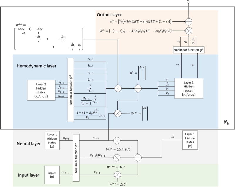
An overview of DCM-RNN
3.2 DCM-RNN parameter estimation
Since all its operators are partial differentiable, DCM-RNN can be trained by TBPTT. We first find the MAP estimation of θ and then calculate the free energy bound with the Laplace approximation post hoc. Assume the observation noise z and the prior distribution of θ for a given model are both Gaussian,
| (39) |
| (40) |
where g1:T is the outputs of hemodynamic function g for all time points. Eq. (39)(40) lead to
| (41) |
where εy = y − g1:T (θ) and εp = θ − μp. Ny = TNb is the total number of fMRI values. Σ accounts for the temporal and spatial correlation of the observation noise and takes a restricted form to constrain its degrees of freedom
| (42) |
where θλ = {λi|i = 1, 2,…} is the DCM hyper parameters and are predefined covariance matrix patterns (Friston, 2002). The loss function l(θ) of DCM-RNN is set as − ln p(θ|y, m) after removing the constant terms
| (43) |
where εy, εp, and Σ are functions of θ. The optimization objective of l(θ) is essentially equivalent to the one for DCM described in Eq.(20).
3.3 Implementation of DCM-RNN on deep learning platform
In this section, we highlight some important details of our DCM-RNN implementation on Tensorflow (GoogleResearch, 2015), an open source deep learning platform supported by Google. It uses a variant of TBPTT for RNN parameter tuning. Instead of a complete unfolded RNN, matching the whole length of target signals, Tensorflow unfolds a RNN to a fixed length, which is short and closely related to the back propagation length in TBPTT. It balances computation and the model’s long-term correlation capturing ability. After building the short model, Tensorflow cuts training signals into (overlapping) segments and stacks segments from different samples into a batch. Segments in a batch are of the same time index. Gradients from the segments in a batch are calculated in parallel. The gradient used to update a parameter is the mean or the sum of gradient from all segments in the batch. It is the standard multi-sample parallelism. It speeds up the computation and stabilizes parameter tuning. Typically, model parameters are updated after each batch. Tensorflow respects the temporal dependency of batches. For each batch, the initial values of the hidden states are read from its preceding batch. It means parameter updating for a batch depends on parameter updating of its preceding batches.
The unfolding length is crucial for DCM-RNN and tends to be longer than the ones usually used for a classic RNN. On one hand, since input at one time point may affect the BOLD signal in the coming seconds, according to our rule of thumb, the unfolded DCM-RNN should cover a comparable or longer range, such as 8 seconds. Otherwise, the gradient obtained by TBPTT is not reliable and does not point to the right direction. On the other hand, the time interval between adjacent time points Δt needs to be small to validate the Euler’s approximation. According our experiments, Δt = 1/16 second seems an appropriate choice. Consequently, the unfolded DCM-RNN should be no shorter than 128 time points.
The multi-sample parallelism is not applicable in DCM-RNN when we infer an interesting objective for a single subject with a single time series. The loss of the multi-sample parallelism leaves the DCM-RNN estimation slow and the gradient calculation instable. We develop a single-sample parallelism to attenuate the problems. At the beginning of each epoch, we use the parameters determined in the previous epoch to run a forward pass of DCM-RNN, namely simulating the whole fMRI sequence, to obtain the values of the hidden states at each time point. After cutting the single time series into segments, we stack every 128 segments from the same sample into a batch and feed it into Tensorflow. Tensorflow will calculate gradients from the segments in the batch in parallel. The initial values of the hidden states for each segment come from the initial forward pass at the beginning of the epoch. We sum up gradients from all the batches and do a global updating of the model parameters. The singlesample parallelism detaches the temporal dependency of parameter updating but not the temporal dependency of the signals. Drop out can be used to randomly skip the gradient calculation for a percentage of the segments to further decreases the computation load. In our experiments, this parallelism leads to more than 10X speed up and enhances stability of parameter tuning.
Choosing a proper step size for parameter updating is tricky in DCM-RNN. The proper step size depends on many factors such as segment length, number of brain regions, fMRI signal magnitude, Δt, etc. The proper step size at the beginning of training can also be very different from the one at the end of a training. Instead of a fixed step size, in each epoch, we use adaptive step size so that the product of the step size and the maximal gradient magnitude among all the parameters equals to a constant. If an updating increases the loss value, we further decrease the step size, which is typically known as backtracking in optimization. A similar backtracking device is used in the Statistical Parametric Mapping (SPM) implementation of DCM, based on an abbreviated gradient descent and the matrix exponential form of the local linearization. Sometimes, after back tracking several times, DCM-RNN still cannot reduce the loss. It may be caused by two reasons: the step size is still too large, or the current gradient is not accurate. Since each segment only sees a short duration of the whole signal, the gradients calculated from segments may be different from the global optimal. Averaging the segment gradients are likely to reduce the error but not likely to eliminate it completely. The inaccuracy of the gradient may also result from random drop out of signal segments. Without inferring the exact reason, we abandon the current gradient and reduce the updating constant, i.e. the product of the step size and the maximal gradient magnitude, which systematically reduces the step size in all following iterations.
4 Experiments
4.1 General settings
The main widely-used DCM implementation is in Statistical Parametric Mapping (SPM). In our experiments, we use SPM 12, the latest released version of SPM, and we will refer to it as DCM-SPM. Several peripheral modifications are made to the released DCM-SPM codes to make the implementation match the theory discussed in this paper. In spm_dcm_estimate, fMRI signal is not detrended and not rescaled. In spm_fx_fmri, P.A is not log self-inhibited and C is not rescaled to 1/16 of its original value. In spm_dcm_fmri_priors, the prior mean of the off-diagonal entries in A is set to zero, instead of 1/128 to prevent it from biasing toward positive value in parameter estimation. DCM-SPM provides several options of integration schemes to discretize DCM. We use spm_int_J, because it uses an explicit Jacobian-based update rule that is infallible and preserves nonlinearities in DCM, although it runs much slower than the default spm_int.
Functional MRI data are up sampled to meet the requirement of Δt in both models and fMRI signals are further cut into segments in DCM-RNN for TBPTT. They change the number of data points while the prior terms in the optimization objective in both models does not scale with data. Thus, we rescale the prior covariances to keep the models well-regulated during optimization. The variances are rescaled by two factors: the first is up sampling factor, calculated as the original fMRI temporal resolution divided by the up sampled fMRI temporal resolution; the second is segmentation factor, calculated as the original fMRI temporal length divided by the segment length and the batch size. For DCM-SPM, the segmentation factor is 1. After finding a MAP estimator of DCM parameters, we calculate the 90% confidence range for each parameter to evaluate the uncertainty of the estimation and the free energy as a metric of fitting goodness. The confidence range and the free energy are calculated based on the Laplace approximation using DCM-SPM routines. For DCM-RNN, we feed the MAP estimator into DCM-SPM routines. Notably, fMRI signals in DCM-RNN are only cut into segments during the MAP estimation phase, not the confidence range and free energy evaluation, and thus the segmentation prior rescaling factor is not applied. It ensures a fair comparison between DCM-RNN and DCM-SPM. The fMRI signal up sampling also has a direct influence on the confidence range and the free energy, because the added pseudo samples make the system overconfident in the estimation as if it had more observations than it actually did. For example, if fMRI signal is up sampled by a factor of two, the confidence range and the free energy will be half of their original values, given other terms in the object function properly rescaled accordingly. The overconfidence has been corrected in the reported confidence range and free energy. We do not compare the free energy bound on model evidence in noise free experiments because this would require an estimation of accuracy - and the accuracy is not well defined in the absence of observation noise.
In all experiments with simulated data, fMRI signals are generated with DCM-RNN and DCM-SPM respectively. Estimations are done with their own simulated data to avoid potential bias. The original simulated data with 1/64 second interval are down sampled to 2 seconds interval, simulating fMRI acquisition process, and then up sampled to 1/16 second interval. Identical and independently distributed (i.i.d.) Gaussian noise is added to the down sampled signals with signal to noise ratio (SNR) being {5, 3, 1}, which are the typical values for fMRI. SNR is defined as the ratio of the standard deviation of BOLD signal and the standard deviation of the noise. In estimation, settings in DCM-SPM are kept as default if not otherwise stated and DCM-RNN is matched to DCM-SPM. The initial values of A is a negative identity matrix, and BC are zero matrices. This initialization only uses the prior knowledge that node self-loop should provide negative feedback as required by system stability. θh is initialized as its prior mean. Parameters are independently distributed in prior. The prior mean and the prior variance in DCM-RNN are summarized in Table 2. Note that in DCM-SPM, {κ, τ, ε} and {f, v, q} are protected with an exponent transform to prevent them from running into negative values. In the presented experiments, such a problem does not occur in DCM-RNN and we do not adopt the transform in DCM-RNN for the moment. It will be added in further implementation. One covariance pattern Q is used for each brain region, which is a diagonal matrix. It essentially assumes that the observation noise is temporally and spatially uncorrelated, but the noise strength can be different for different regions. All parameters [θC, θh, θλ] are updated during estimation. Variational Bayes with Gauss-Newton search is used for parameter estimation for DCM-SPM as in spm_nlsi_GN. In spm_nlsi_GN, the initial log ascent rate is decreased to −10 to prevent algorithm crashing caused by aggressive parameter updating.
Table 2.
Prior mean and variance before rescaling
| Variable | Mean | Variance |
|---|---|---|
| A | 0 | 1/64 |
| B | 0 | 1 |
| C | 0 | 1 |
| κ | 0.64 | 1/256 |
| γ | 0.32 | 0 |
| τ | 2 | 1/256 |
| E0 | 0.4 | 0 |
| α | 0.32 | 0 |
| V0 | 4 | 0 |
| θ0 | 40.3 | 0 |
| r0 | 25 | 0 |
| ε | 1 | 1/256 |
| λ | 6 | 1/128 |
• Zero variance of a variable means the variable is kept constant during parameter estimation as its mean
• If a variable is a vector or matrix, expectation and variance listed above are for each entry in the vector or matrix.
All the estimation experiments are carried out on a Macintosh laptop with an Intel Core i5 processor and 16 GB memory. No graphic processor unit is used. We report running time of the two models, which reflects the current development of the two models but not a formal speed comparison since neither of the two model implementations is optimized for speed. For DCM-RNN, we do not count the time building a Tensorflow computation graph because it needs to be done only once and can be used for all experiments. Relative root mean square error (rRMSE) is used to compare similarity between variables, which is defined as the l2 norm of the difference between two variables divided by the l2 norm of the anchor variable in the two, which is usually the ground truth one. All the codes used in the experiments, including the DCM-RNN and the modified DCM-SPM codes, are available online at https://github.com/YuanWangOnward/DCM_RNN.
4.2 The impact of Δt
Euler’s method of integration approximation requires a small Δt. To evaluate the impact of Δt, we simulate fMRI signals with 10,000 different DCM parameter configurations and compare the signals obtained with different Δt in each configuration. The generation of the configurations is random, including the number of brain regions, the number of stimuli, the stimulus functions, θC and θh. However, not every random configuration can generate realistic fMRI signals, even if A is ensured to be a stable transition matrix. We filter out the unqualified ones by checking the maximum absolute value, the mean, and the variance of x, and the maximum and the minimum values of {s, f, v, q}. The criteria are chosen heuristically to avoid exploding and vanishing fMRI signals. The 10,000 configurations are the ones that survived the above criteria. In each configuration, fMRI signals generated with Δt = 1/64 second serves as the ground truth and others with Δt = {1/32, 1/16, 1/8, 1/4, 1/2} second are compared against it. In each comparison, the ground truth signal is down sampled to the lower temporal resolution and compared with the signal generated at the lower temporal resolution.
Fig. 7 shows three examples of fMRI signals generated using the DCM-RNN with randomly generated DCM configurations. The generated examples are realistic in the sense that they fluctuate with the inputs, without exploding or vanishing.
Fig. 7.
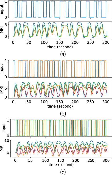
Three examples of fMRI signals simulated by random DCM configurations. (a) 1 stimulus and 3 fMRI signals. (b) 2 stimuli and 4 fMRI signals. (c) 3 stimuli and 5 fMRI signals.
Fig. 8 shows the histograms of the simulation errors with different Δt and Table 3 summarizes the mean and the deviation of each histogram. As predicted by error estimation for Euler’s method, the smaller the Δt is, the smaller the simulation error is. Δt = 1/32 second can almost ensure the whole rRMSE histogram is within 5% and the expectation of rRMSE with Δt = 1/16 second is within 5%. For a DCM-RNN covering a fixed length of time, its time complexity is O(1/Δt). It means as Δt approaches 0, the computation increases extremely fast. To balance between accuracy and computation, we use Δt = 1/16 second in the following experiments unless otherwise stated.
Fig. 8.
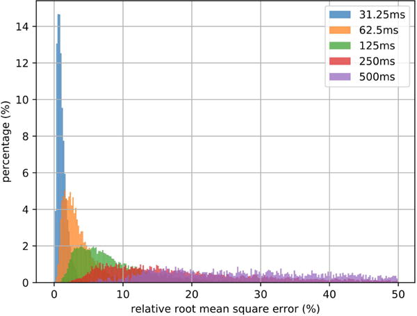
Histograms of simulation rRMSE with different Δt.. The histograms are normalized so that each sums to 1.
Table 3.
Mean and variance of simulation rRMSE for various Δt.
| Δt (second) | Mean | Standard deviation |
|---|---|---|
| 1/32 | 1.20% | 0.690% |
| 1/16 | 3.58% | 2.24% |
| 1/8 | 9.14% | 6.24% |
| 1/4 | 27.4% | 29.3% |
| 1/2 | 210% | 271% |
4.3 The impact of up sampling
The experiment on Δt shows that the current standard 2-second interval of fMRI accquisition is too large for the approximation to be valid. One quick fix is to up sample the accquired fMRI data, which may induce error. We perform a down-up sample comparison to evaluate the error. We re-use the fMRI signals generated in the previous experiment with Δt = 1/16 second. The fMRI signals are first down sampled to Δt = 2 seconds, simulating the fMRI acquisition process, and then up sampled with cubic spline interpolation back to Δt = 1/16 second.
Fig. 9 shows the histogram of rRMSE caused by the resampling process. The mean is 0.901% and the standard deviation is 0.336%. It illustrates that the error caused by up sampling is small and stable.
Fig. 9.
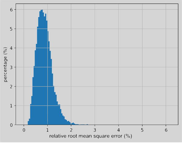
Histograms of errors caused by resampling.
4.4 Effective connectivity estimation with simulated data (study one)
4.4.1 Experimental settings
In this experiment, we will first generate fMRI data with known DCM parameters and evaluate the integration schemes implicit in DCM-SPM and DCM-RNN. We will then validate the two estimates in terms of the posterior expectations and 90% confidence ranges of effective connectivity, with various levels of observation noises. Functional MRI prediction error, connectivity estimation error, free energy, and running time will be included in the comparison.
In simulation, the input is randomly generated box train, θC is set as in Fig. 10. In estimation, the supports of the θC is set as the true ones and Δt = 1/16 second. In DCM-RNN, the length of the unfolded DCM-RNN is 192. Simulated fMRI signals are cut into overlapping segments with segment length 192 and stride 1. The initial maximal parameter updating in each epoch is 0.002 and the maximal backtracking number is 4. Dropout rate is 0%. We run DCM-RNN for 96 epochs before harvesting the results.
Fig. 10.
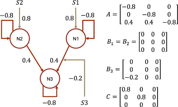
The data generating causal architecture and effective connectivity in study one. N and S indicate brain region/node and stimuli.
4.4.2 Results and discussion
Fig. 11 shows the randomly created input stimuli and the fMRI signal simulated by DCM-RNN and DCM-SPM. Comparing to the DCM-SPM simulation, the rRMSE of the DCM-RNN simulation is 0.482%. It shows that our conversion of DCM to DCM-RNN is faithful. We attribute the small difference to the different integration schemes used in the two models.
Fig. 11.
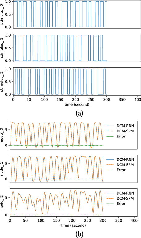
Functional MRI simulation. (a) shows the random inputs. (b) shows the simulated fMRI signals by DCM-RNN and DCMSPM and the difference between the two.
Fig. 12 shows the estimation results with noisy fMRI, SNR=5. The blue solid curves in Fig. 12 (a)(b) show the resampled fMRI signals, which is used as the observed fMRI signals for parameter estimation. The resampling of fMRI induces 1.16% rRMSE in DCM-RNN and 1.00% rRMSE in DCM-SPM. These are the errors of predicted fMRI signals with the ground truth parameters. The orange dashed curves in in Fig. 12 (a)(b) show the predicted fMRI with the estimated parameters. Fig. 12 (c) shows a bar plot of the estimated effective connectivity values with 90% confidence range. Fig. 13 shows the estimation results with SNR=1. The figure presentation is analogous to Fig. 12.
Fig. 12.
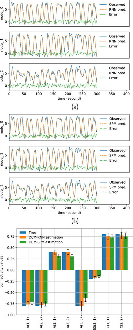
Estimation results with noisy simulation, SNR=5. (a)(b) show the resampled fMRI signals as ‘Observed’ and the predicted fMRI signals with estimated parameters for DCM-RNN and DCM-SPM (c) shows the estimated connectivity parameters with 90% confidence range.
Fig. 13.
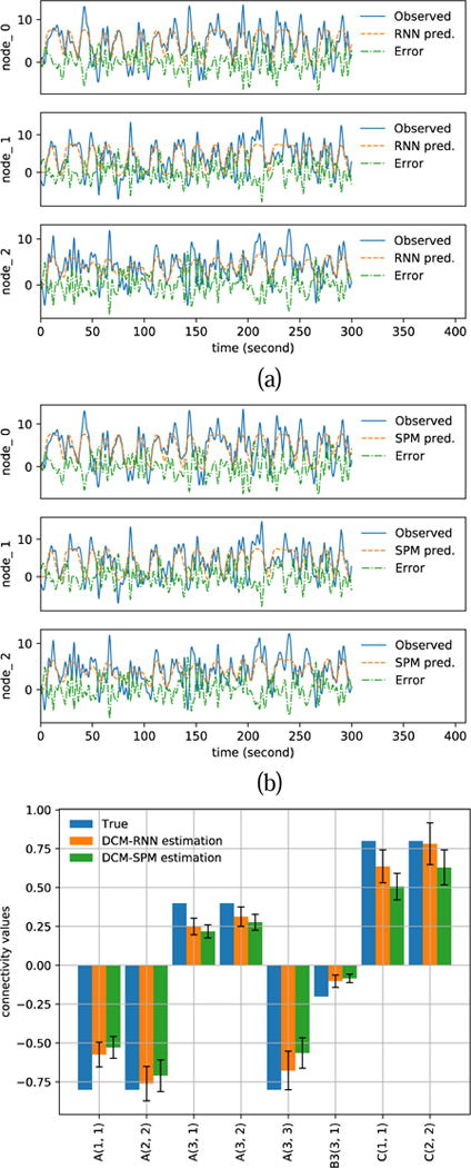
Estimation results with noisy simulation. SNR=1. (a)(b) show the resampled fMRI signals as ‘Observed’ and the predicted fMRI signals with estimated parameters for DCM-RNN and DCM-SPM. (c) shows the estimated connectivity parameters with 90% confidence range.
Numerical results are summarized in Table 4. For all levels of noise, DCM-SPM tends to have smaller fMRI reproduction errors. However, the connectivity errors of DCM-SPM are significantly higher than DCM-RNN. It suggests that DCM-SPM converges to a local minimal other than the ground truth point in the parameter space. The accuracy of connectivity estimation of DCM-RNN is also supported by its higher free energy values. On average, DCM-SPM ran 21.0 iterations which took 20.5 minutes, DCM-RNN ran fixed 96 epochs (iterations) which took 139.8 minutes.
Table 4.
Results of effective connectivity estimation, study one.
| Model | SNR | fMRI rRMSE |
Connectivity rRMSE |
Free energy |
|---|---|---|---|---|
| RNN | Noiseless | 1.82% | 1.01% | / |
| SPM | Noiseless | 1.08% | 8.39% | / |
| RNN | 5 | 9.83% | 3.96% | −2.52e+03 |
| SPM | 5 | 9.78% | 13.8% | −2.61e+03 |
| RNN | 3 | 15.4% | 7.16% | −3.84e+03 |
| SPM | 3 | 15.2% | 17.0% | −3.94e+03 |
| RNN | 1 | 43.8% | 19.4% | −8.26e+03 |
| SPM | 1 | 43.5% | 29.7% | −8.69e+03 |
This experiment shows that the effective connectivity can be estimated by back propagation. It is a demonstration that DCM-RNN can be used to infer biophysical objective in a neural-network friendly way.
4.5 Effective connectivity estimation with simulated data (study two)
4.5.1 Experimental settings
In this experiment, we use a more challenging causal architecture, which consists of reciprocal connectivities as in Fig. 14. The architecture has been studied in (Friston et al., 2003). Other experimental settings stay the same as in study one, except that we run DCM-RNN for 128 epochs before harvesting the results.
Fig. 14.
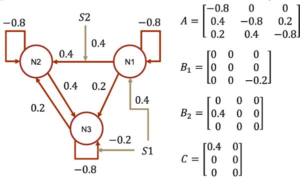
The data generating causal architecture and effective connectivity in study two. N and S indicate brain region/node and stimuli. This architecture has been studied in (Friston et al., 2003).
4.5.2 Results and discussion
The figure presentation of Fig. 15 to Fig. 17 is analogous to Fig. 11 to Fig. 13. Compared to the DCM-SPM simulation, the rRMSE of the DCM-RNN simulation is 0.476%. The resampling of fMRI induces 0.775% rRMSE in DCM-RNN and 0.478% rRMSE in DCM-SPM. Numerical results are summarized in Table 5. It is interesting to see that DCM-RNN did not do well in the noiseless case but better in the cases with small noise. We think it is because DCM-RNN got stuck in a flat area of the cost landscape, potentially a saddle point, and was not able to reach an optimal point before the optimization stopped. It is known that saddle points can significantly slow down gradient descent and noise can help the gradient descent algorithm to escape saddle points (Ge et al., 2015). Saddle point is less a problem for DCM-SPM because its Gauss-Newton search uses local curvature to scale the step size which help to escape saddle points efficiently. In the noiseless case, DCM-SPM ran 26 iterations which took 34.3 minutes and DCM-RNN ran fixed 128 epochs (iterations) which took 348.0 minutes. In other cases, on average, DCM-SPM ran 22.0 iterations which took 28.3 minutes and DCM-RNN ran fixed 128 epochs (iterations) which took 229.2 minutes. The running time of both models is significantly longer in noiseless case than in noisy cases. It supports our hypothesis that there may be some ill conditioned points (potentially saddle points) on the path from the initial point to the ground truth point in the parameter space. In the neighborhood of the points, the two models have to adjust the step size through back tracking frequently which slows down the estimation process. Noise appears to help the models escape from the ill conditioned points. The running time in this experiment is longer than the previous experiment, especially for DCM-RNN for the following reasons: 1) The total scan time is 6 minutes in this experiment and 5 minutes in the previous experiment. 2) DCM-RNN ran 128 epochs in this experiment and 96 epochs in the previous experiment. 3) The loss landscape in this experiment seems to be harder to optimize on so that the models have to adjust step size very often.
Fig. 15.
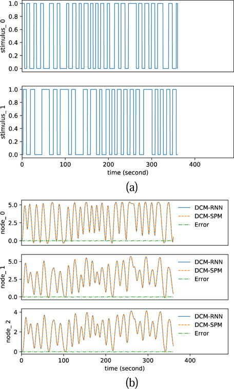
Functional MRI simulation. (a) shows the random inputs. (b) shows the simulated fMRI signals by DCM-RNN and DCM-SPM and the difference between the two.
Fig. 17.
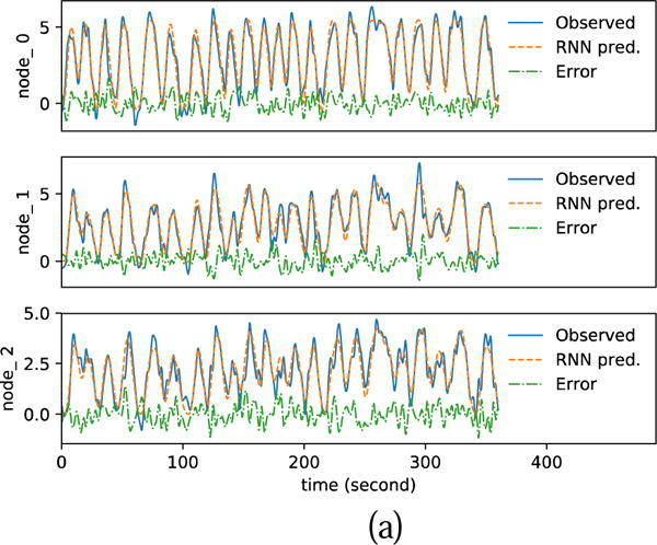
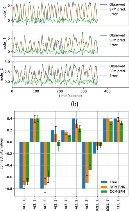
Estimation results with noisy simulation. SNR=3. (a)(b) show the resampled fMRI signals as ‘Observed’ and the predicted fMRI signals with estimated parameters for DCM-RNN and DCM-SPM. (c) shows the estimated connectivity parameters with 90% confidence range.
Table 5.
Results of effective connectivity estimation, study two.
| Model | SNR | fMRI rRMSE |
Connectivity rRMSE |
Free energy |
|---|---|---|---|---|
| RNN | Noiseless | 5.13% | 17.5% | / |
| SPM | Noiseless | 0.621% | 14.8% | / |
| RNN | 5 | 9.91% | 12.1% | −1.57e+03 |
| SPM | 5 | 9.68% | 27.0% | −1.67e+03 |
| RNN | 3 | 15.5% | 13.2% | −2.73e+03 |
| SPM | 3 | 15.3% | 32.9% | −2.92e+03 |
| RNN | 1 | 41.8% | 22.5% | −6.42e+03 |
| SPM | 1 | 41.5% | 38.2% | −6.73e+03 |
Major observations are consistent with the previous experiment. DCM-SPM tends to have smaller fMRI reproduction errors but higher connectivity errors and lower free energy values. It is another evidence that DCM-RNN and back propagation can be used to infer biophysical quantities such as the effective connectivity.
4.6 Model selection with simulated data
4.6.1 Experimental settings
In this experiment, we try to identify the most plausible causal architecture among hypothesis candidates. The data generating causal architecture and the two competing hypotheses are abstracted from the model selection demo in the SPM12 manual chapter 35 “Dynamic Causal Modeling for fMRI”. The architectures have forward and backward connectivities representing reciprocal interactions which are known to play an important role for brain functional integration. We create five subjects in the experiment. The subjects have different hemodynamic parameters which are randomly sampled from the prior distribution of θh. Because of number of samples is small (i.e. 5), we constrain the sampling to 90% confidence range to avoid extreme samples. We use identical θC for the five subjects without random sampling, because the prior of θC is not biophysically informed and random sampling from it does not reflect inter-subject heterogeneity. Free energy values are calculated per subject and per model. They are used as the individual level statistics and fed into group level model comparison using the exceedance probability (Stephan et al., 2009) which measures the posterior probability that one model is preferred than any other model. The exceedance probability is calculated using spm_BMS.
The data generating causal architecture is shown in Fig. 18 and the two competing architecture hypotheses are shown in Fig. 19. The two hypotheses differ in the modulation of the third stimulus. In the first hypothesis, the third stimulus modulates a backward connectivity from N3 to N2; in the second hypothesis, it modulates a forward connectivity from N1 to N2. In simulation, the input is designed box trains exploring the input space. Before model inversion, the simulated signals are down-up sampled and i.i.d. Gaussian noise is added with SNR=3. Other experimental settings are the same as in effective connectivity estimation study one.
Fig. 18.
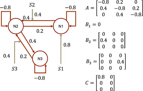
The data generating causal architecture and effective connectivity in model selection experiment. N and S indicate brain region/node and stimuli. This architecture has been studied in the model selection demo in the SPM12 manual chapter 35 “Dynamic Causal Modeling for fMRI”
Fig. 19.
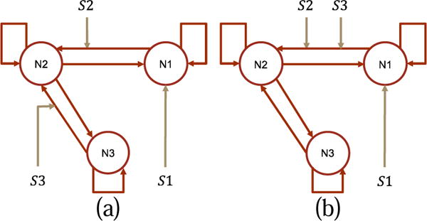
The two hypotheses in the model selection experiment. (a) hypothesis zero. (b) hypothesis one. The hypotheses differ in the modulation of the third stimulus. These hypotheses have been studied in the model selection demo in the SPM12 manual chapter 35 “Dynamic Causal Modeling for fMRI”
4.6.2 Results and discussion
Fig. 20 shows the inputs and the fMRI signals simulated by the two models for one subject. Fig. 21 and Fig. 22 show the estimated effective connectivity for two representative subjects. Although the connectivity B3(2, 1) does not exist in the true architecture, it can have a nontrivial value if incorrectly supported as in hypothesis one. Large confidence ranges of connectivity A(2, 3) crossing zero reflect large uncertainty in the estimation. For some subjects, the A(2, 3) estimation ended up with a wrong sign in DCM-SPM. Such a sign error did not occur in DCM-RNN. Fig. 23 shows the free energy comparison between hypotheses. For all the subjects, the free energy value is higher in hypothesis zero than in hypothesis one. The average free energy difference between hypotheses is 198.6 in DCM-SPM and 258.8 in DCM-RNN, which mean DCM-RNN is more sensitive to hypothesis difference. The exceedance probability of hypothesis zero is 0.984% for both of the models, hitting the maximum output of spm_BMS. It means hypothesis zero, which is the true data generating architecture, is overwhelmingly favored in both models. This is a demonstration of DCM-RNN face validity with regard to model selection.
Fig. 20.
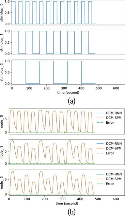
Functional MRI simulation. (a) shows the inputs. (b) shows the simulated fMRI signals by DCM-RNN and DCM-SPM and the difference between the two. It is the simulation for one subject.
Fig. 21.
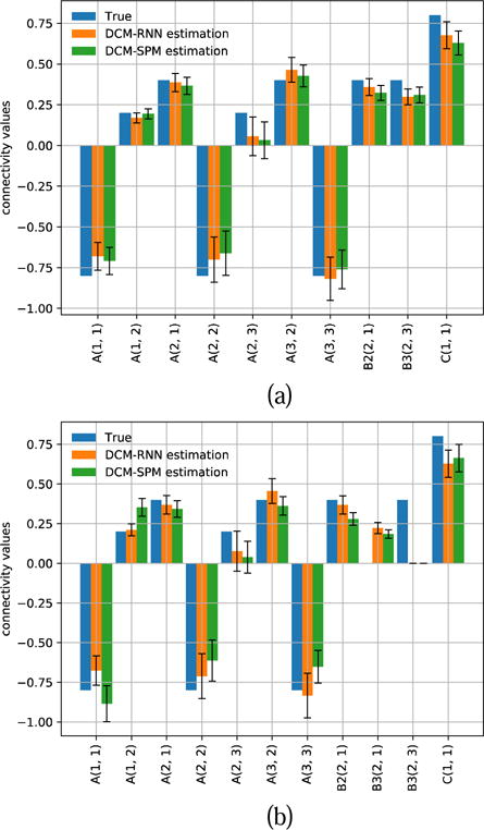
Estimated connectivity with 90% confidence range for one representative subject. (a) shows the result of hypothesis zero. (b) shows the result of hypothesis one.
Fig. 22.
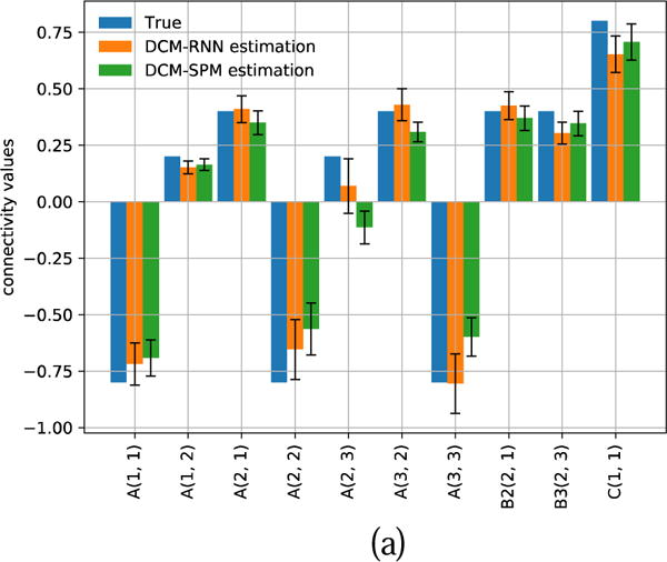
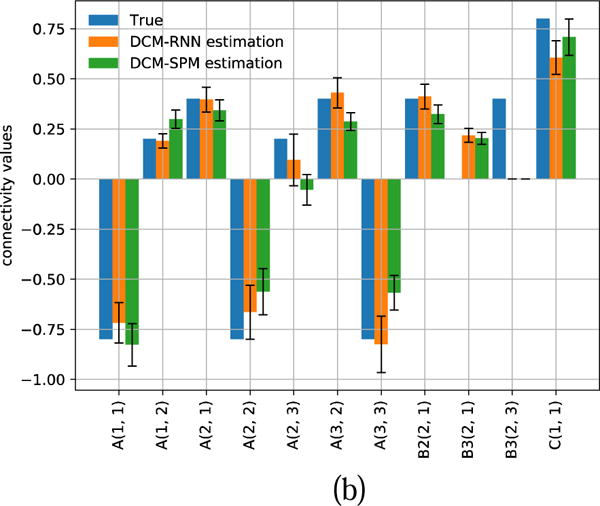
Estimated connectivity with 90% confidence range for another representative subject. (a) shows the result of hypothesis zero. (b) shows the result of hypothesis one.
Fig. 23.

Free energy value comparison between the two competing hypotheses.
4.7 Effective connectivity estimation with real fMRI data
4.7.1 Experimental paradigm
Details of the experimental paradigm and the fMRI acquisition can be found in (Büchel and Friston, 1997). The purpose of the experiment is to evaluate the modulatory effect of attention. Visual stimuli are projected onto a screen with a fixation point at the center. Visual content contains dots moving from the centered fixation towards the screen boundary where they vanish. During certain periods, subjects are instructed to try to detect a change in speed of the dots and otherwise to ‘just look’. The preprocessed data can be found on the SPM website under the name of ‘Attention to Visual Motion fMRI data set’. The data set is smoothed, spatially normalized, realigned, slice-time corrected with SPM99.
4.7.2 Experimental settings
A DCM study is setup following the example in the SPM12 manual. There are three 0–1 box train inputs. If the visual content is present on the screen, the photic input is on; if the dots are moving, the motion input is on; if the subjects are instructed to detect dots speed change, the attention input is on. Three brain regions that are believed to be engaged during photic stimulation are included: V1, the primary visual cortex; V5, the middle temporal visual area responsible for motion perception; and superior parietal cortex (SPC). V5 and SPC are believed to be engaged during attention. The locations of the regions are identified by the general linear model (GLM) as the highest correlated points. Each region is a sphere with radius 8mm centered at V1(0, −93, 18), V5(−36, −87, −3), and SPC(−27, −84, 36) in the standard space as shown in Fig. 24. The support of the causal architecture is set as in Fig. 25.
Fig. 24.
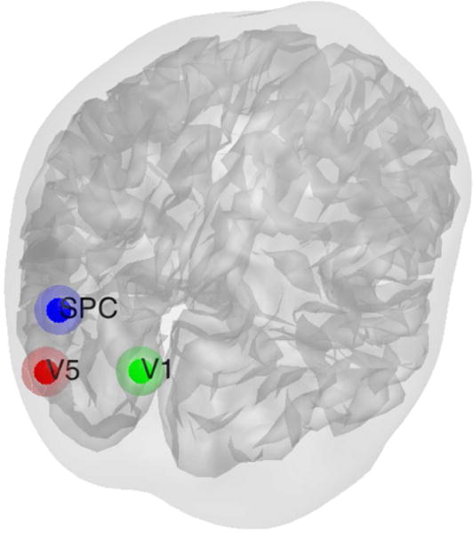
Locations of brain regions included in the attention experiment.
Fig. 25.

Support pattern of the DCM study in the attention experiment.
An extra linear component is added to the hemodynamic function to account for the influence of baseline drifting or other low frequency non-neural fluctuations in the measured data. For the n-th region,
| (44) |
where G is the confound matrix, whose columns are the first 19 Discrete Cosine Transform (DCT) bases. β is a weight vector for the confounds. In DCM-RNN, θ and β are updated iteratively. The linear component is the default setting in DCM-SPM and 19 is the default value. In DCM-RNN, the length of the unfolded DCM-RNN is 256. Simulated fMRI signals are cut into overlapping segments with segment length 256 and stride 2. The initial maximal parameter updating in each epoch is 0.005 and the maximal backtracking number is 4. Dropout rate is 25%. We run DCM-RNN for 128 epochs before harvesting the results.
4.7.3 Results and discussion
Fig. 26 shows estimation results with real fMRI. Compared to the observed fMRI signal, the fMRI prediction error is 56.8% for DCM-RNN and 56.0% for DCM-SPM. Given the noise level, the prediction accuracy of the two models are very similar. The free energy is −3.01 × 10³ for DCM-SPM and −3.26 × 10³ for DCM-RNN. DCM-SPM ran 44 iterations before convergence which took 5.57 hours; DCM-RNN ran 128 epochs (iterations) which took 7.76 hours. All the estimated connectivity values by the two models have the same signs and the majority of them are qualitatively similar. DCM-SPM indicated a very strong backward influence from SPC to V5 and then V1, while DCM-RNN tends to use fewer significant non-zero connectivities. Foremost, the two models agreed on that attention had a positive influence on the backward connectivity from SPC to V5.
Fig. 26.

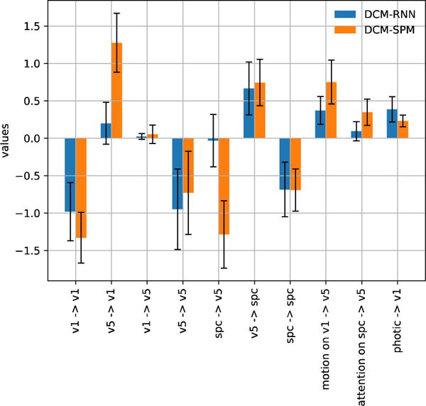
Estimation with real fMRI data. (a) shows the three inputs. (b) shows the predicted fMRI signals with estimated parameters. (c) shows the estimated connectivity.
5 Discussion
In this paper, we focus on the original DCM (Friston et al., 2003). It is interesting to consider how other DCM variants may fit into DCM-RNN framework. The nonlinear DCM (Stephan et al., 2008) uses a quadratic form of the neural evolution equation where the quadratic term indicates the influence of the neural activity of one brain region on other connectivities. It can be achieved in DCM-RNN by augmenting ϕx with quadratic terms of x and adding corresponding coefficients in Wxx and Wxxu. The multiple neural states DCM (Marreiros et al., 2008) incorporates two neural states per region, which models the activity of an inhibitory and an excitatory population respectively. It can be achieved in DCM-RNN by splitting x into [xexcitatory, xinhibitory] for each brain region and enlarging Wxx and Wxxu accordingly. A hierarchical DCM can be found in (K. Friston, 2008)(Friston et al., 2010)(Friston et al., 2008) where the hierarchy is built on the temporal derivatives of DCM states. In DCM-RNN, it can be achieved by augmenting x into and modifying the weighting matrices W properly: specifying the block structure and parameter sharing in W. In (Seghier and Friston, 2013), the prior covariance of A is derived from the observed fMRI signals to reduce the effective number of free parameters to enable DCM studies with large number of nodes. In DCM-RNN, one can simply change the corresponding part in Σp with the derived covariance for A.
Stochastic DCMs (Friston et al., 2008)(K. J. Friston, 2008)(Friston et al., 2010) assume a random fluctuation in the neural activity space which means one has to estimate the true neural states together with DCM parameters. Conceptually, one can absorb the states into parameters, treating the state value at each time point as a separate parameter. Obviously, the state parameters are highly correlated because of the neural evolution equation. Similar unification has been used in (Friston et al., 2010) where all parameters are absorbed into states. Denote the augmented parameter set as Θ. Incorporating the stochastic DCMs into DCM-RNN framework means being able to estimate the posterior distribution of Θ. Treatments of variational Bayes in DNN/RNN framework has been proposed in (Kingma and Welling, n.d.)(Fabius and van Amersfoort, n.d.). Briefly, one can declare the parameters of the posterior distribution of Θ as trainable variables in a DCM-RNN and then do the following steps iteratively until convergence: 1) randomly draw samples of Θ from the posterior distribution and calculate the loss values for the samples. 2) back propagate the loss to the parameters of the posterior distribution. In practice, one may want to assume properties of the posterior distribution of Θ, such as independence between subsets of Θ and state transition p(xt+1|xt) indicated by the state evolution equations.
DCM has two variants tailored for rsfMRI (Friston et al., 2014a)(Friston et al., 2014b). The spectral DCM (Friston et al., 2014a) works in the frequency domain where the unknown stimuli can be parameterized very efficiently based on the power law. The spectral DCM predicts the cross spectra among observed fMRI signals instead of the raw values of fMRI signals. In (Friston et al., 2014b), the effective connectivities are further parameterized by eigenmodes and Lyapunov exponents, where the eigenmodes are derived from functional connectivity. In DCM-RNN, it is easy to parameterize the effective connectivities by eigenmodes and their Lyapunov exponents. Since the eigenmodes are derived from functional connectivity and fixed, one can declare the Lyapunov exponents as trainable variable and back propagate errors to the exponents. DCM-RNN is a time domain model in nature, but it does not mean it cannot use frequency information. One can parameterize the unknown stimuli in rsfMRI as a linear combination of DCT bases and tune the combination weightings with back propagation. This representation has been used in (Friston et al., 2011). The prior distribution of the combining weightings can be configured according to the power law. One can add a layer on top of DCM-RNN which takes predicted fMRI signals as input and outputs the cross spectra. A loss can be defined as the difference between the predicted cross spectra and the observed cross spectra and back propagation can be used to tune the model parameters, including the DCT weightings and the effective connectivity, to minimize the loss.
6 Conclusions
In this paper, we propose a biophysically interpretable RNN, DCM-RNN. It casts the advanced biophysical model, DCM, into a generalized RNN. The conversion is faithful without loss of any biophysical significance of the original DCM. The hidden states of DCM-RNN are neural activity, blood flow, blood volume, and deoxyhemoglobin content and parameters of DCM-RNN are biological quantities such as effective connectivity, oxygen extraction fraction at rest and vessel stiffness. Through experiments with both simulated and real fMRI data, we demonstrate that DCM-RNN with back propagation is valid for DCM parameter estimation. It paves the way to DCM studies with complex stimuli and DNN-based representation.
Fig. 16.
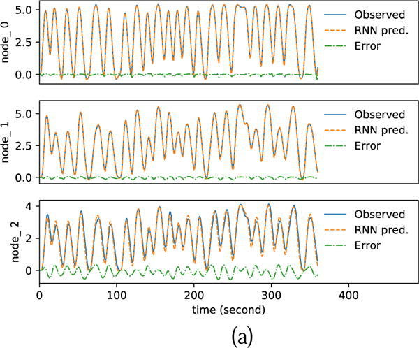
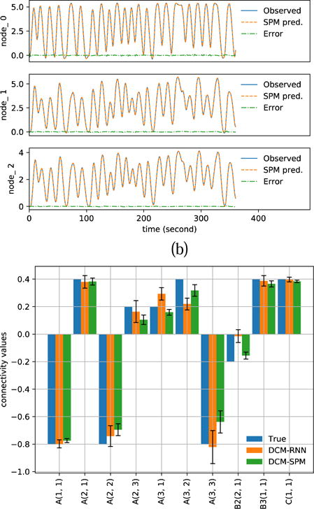
Estimation results with noiseless simulation. (a)(b) show the resampled fMRI signals as ‘Observed’ and the predicted fMRI signals with estimated parameters for DCM-RNN and DCM-SPM (c) shows the estimated connectivity parameters with 90% confidence range.
Acknowledgments
This work is supported in part by grant funding from the National Institutes of Health (NIH): R01 NS03913511 and R21 NS090349, National Institute for Neurological Disorders and Stroke (NINDS). This work is also performed under the rubric of the Center for Advanced Imaging Innovation and Research (CAI2R, www.cai2r.net), a NIBIB Biomedical Technology Resource Center (NIH P41 EB017183).
Footnotes
Publisher's Disclaimer: This is a PDF file of an unedited manuscript that has been accepted for publication. As a service to our customers we are providing this early version of the manuscript. The manuscript will undergo copyediting, typesetting, and review of the resulting proof before it is published in its final citable form. Please note that during the production process errors may be discovered which could affect the content, and all legal disclaimers that apply to the journal pertain.
References
- Achille A, Soatto S. Emergence of Invariance and Disentanglement in Deep Representations. JMLR. 2018 preprint. [Google Scholar]
- Aponte EA, Raman S, Sengupta B, Penny WD, Stephan KE, Heinzle J. mpdcm: A toolbox for massively parallel dynamic causal modeling. J Neurosci Methods. 2016;257:7–16. doi: 10.1016/j.jneumeth.2015.09.009. [DOI] [PubMed] [Google Scholar]
- Barak O. Recurrent neural networks as versatile tools of neuroscience research. Curr Opin Neurobiol. 2017;46:1–6. doi: 10.1016/j.conb.2017.06.003. [DOI] [PubMed] [Google Scholar]
- Bengio Y, Courville A, Vincent P. Representation learning: A review and new perspectives. IEEE Trans Pattern Anal Mach Intell. 2013;35:1798–1828. doi: 10.1109/TPAMI.2013.50. [DOI] [PubMed] [Google Scholar]
- Büchel C, Friston KJ. Modulation of connectivity in visual pathways by attention: cortical interactions evaluated with structural equation modelling and fMRI. Cereb Cortex. 1997;7:768–778. doi: 10.1093/cercor/7.8.768. [DOI] [PubMed] [Google Scholar]
- Buxton RB, Wong EC, Frank LR. Dynamics of blood flow and oxygenation changes during brain activation: The balloon model. Magn Reson Med. 1998;39:855–864. doi: 10.1002/mrm.1910390602. [DOI] [PubMed] [Google Scholar]
- Cho K, Van Merriënboer B, Gulcehre C, Bahdanau D, Bougares F, Schwenk H, Bengio Y. Learning phrase representations using RNN encoder-decoder for statistical machine translation. arXiv Prepr arXiv. 2014;1406:1078. [Google Scholar]
- Chumbley JR, Friston KJ, Fearn T, Kiebel SJ. A Metropolis-Hastings algorithm for dynamic causal models. Neuroimage. 2007;38:478–487. doi: 10.1016/j.neuroimage.2007.07.028. [DOI] [PubMed] [Google Scholar]
- Cichocki A, Mandic D, De Lathauwer L, Zhou G, Zhao Q, Caiafa C, PHAN HA. Tensor Decompositions for Signal Processing Applications: From twoway to multiway component analysis. IEEE Signal Process Mag. 2015;32:145–163. doi: 10.1109/MSP.2013.2297439. [DOI] [Google Scholar]
- Daunizeau J, Friston KJ, Kiebel SJ. Variational Bayesian identification and prediction of stochastic nonlinear dynamic causal models. Phys D Nonlinear Phenom. 2009;238:2089–2118. doi: 10.1016/j.physd.2009.08.002. [DOI] [PMC free article] [PubMed] [Google Scholar]
- Bahdana Dzmitry, Bahdanau D, Cho K, Bengio Y. Neural Machine Translation By Jointly Learning To Align and Translate. Int Conf Learn Represent. 2015 doi: 10.1146/annurev.neuro.26.041002.131047. [DOI]
- Fabius O, van Amersfoort JR. Variational recurrent auto-encoders. arXiv Prepr arXiv. 2014;1412:6581. n.d. [Google Scholar]
- Friston K. Hierarchical models in the brain. PLoS Comput Biol. 2008;4:e1000211. doi: 10.1371/journal.pcbi.1000211. [DOI] [PMC free article] [PubMed] [Google Scholar]
- Friston K, Mattout J, Trujillo-Barreto N, Ashburner J, Penny W. Variational free energy and the Laplace approximation. Neuroimage. 2007;34:220–234. doi: 10.1016/j.neuroimage.2006.08.035. [DOI] [PubMed] [Google Scholar]
- Friston K, Stephan K, Li B, Daunizeau J. Generalised filtering. Math Probl Eng. 2010;2010 doi: 10.1155/2010/621670. [DOI] [Google Scholar]
- Friston KJ. Functional and effective connectivity: a review. Brain Connect. 2011;1:13–36. doi: 10.1089/brain.2011.0008. [DOI] [PubMed] [Google Scholar]
- Friston KJ. Variational filtering. Neuroimage. 2008;41:747–766. doi: 10.1016/j.neuroimage.2008.03.017. [DOI] [PubMed] [Google Scholar]
- Friston KJ. Bayesian Estimation of Dynamical Systems: An Application to fMRI. Neuroimage. 2002;16:513–530. doi: 10.1006/nimg.2001.1044. [DOI] [PubMed] [Google Scholar]
- Friston KJ, Harrison L, Penny W. Dynamic causal modelling. Neuroimage. 2003;19:1273–1302. doi: 10.1016/S1053-8119(03)00202-7. [DOI] [PubMed] [Google Scholar]
- Friston KJ, Kahan J, Biswal B, Razi A. A DCM for resting state fMRI. Neuroimage. 2014a;94:396–407. doi: 10.1016/j.neuroimage.2013.12.009. [DOI] [PMC free article] [PubMed] [Google Scholar]
- Friston KJ, Kahan J, Razi A, Stephan KE, Sporns O. On nodes and modes in resting state fMRI. Neuroimage. 2014b;99:533–547. doi: 10.1016/j.neuroimage.2014.05.056. [DOI] [PMC free article] [PubMed] [Google Scholar]
- Friston KJ, Li B, Daunizeau J, Stephan KE. Network discovery with DCM. Neuroimage. 2011;56:1202–1221. doi: 10.1016/j.neuroimage.2010.12.039. [DOI] [PMC free article] [PubMed] [Google Scholar]
- Friston KJ, Mechelli A, Turner R, Price CJ. Nonlinear responses in fMRI: the Balloon model, Volterra kernels, and other hemodynamics. Neuroimage. 2000;12:466–77. doi: 10.1006/nimg.2000.0630. [DOI] [PubMed] [Google Scholar]
- Friston KJ, Trujillo-Barreto N, Daunizeau J. DEM: A variational treatment of dynamic systems. Neuroimage. 2008;41:849–885. doi: 10.1016/j.neuroimage.2008.02.054. [DOI] [PubMed] [Google Scholar]
- Ge R, Huang F, Jin C, Yuan Y. Escaping From Saddle Points - Online Stochastic Gradient for Tensor Decomposition. Conference on Learning Theory. 2015:797–842. [Google Scholar]
- Gonzalez RT, Riascos JA, Barone DAC. How Artificial Intelligence is Supporting Neuroscience Research: A Discussion About Foundations, Methods and Applications. In: Barone DAC, Teles EO, Brackmann CP, editors. Computational Neuroscience. Springer International Publishing; Cham: 2017. pp. 63–77. [Google Scholar]
- GoogleResearch. TensorFlow: Large-scale machine learning on heterogeneous systems 2015 [Google Scholar]
- Graves A, Wayne G, Danihelka I. Neural Turing Machines Arxiv. 2014:1–26. [Google Scholar]
- Grubb RL, Jr, Raichle ME, Eichling JO, T-P M. The effects of changes in PaCO_2 on cerebral blood volume, blood flow, and vascular mean transit time. Stroke. 1974;5:603–609. doi: 10.1161/01.STR.5.5.630. [DOI] [PubMed] [Google Scholar]
- Güçlü U, van Gerven MAJ. Modeling the dynamics of human brain activity with recurrent neural networks. Front Syst Neurosci. 2016:1–19. doi: 10.3389/fncom.2017.00007. [DOI] [PMC free article] [PubMed] [Google Scholar]
- Havlicek M, Friston KJ, Jan J, Brazdil M, Calhoun VD, Havlicek Martin, Firston Karl, jan J. Dynamic modeling of neuronal responses in fMRI using cubature Kalman filtering. Neuroimage. 2011;56:2109–2128. doi: 10.1016/j.neuroimage.2011.03.005. [DOI] [PMC free article] [PubMed] [Google Scholar]
- Hochreiter S, Hochreiter S, Schmidhuber J, Schmidhuber J. Long short-term memory. Neural Comput. 1997;9:1735–80. doi: 10.1162/neco.1997.9.8.1735. [DOI] [PubMed] [Google Scholar]
- Kingma DP, Welling M. Auto-encoding variational bayes. arXiv Prepr arXiv. 1312:6114. n.d. [Google Scholar]
- Marreiros AC, Kiebel SJ, Friston KJ. Dynamic causal modelling for fMRI: A two-state model. Neuroimage. 2008;39:269–278. doi: 10.1016/j.neuroimage.2007.08.019. [DOI] [PubMed] [Google Scholar]
- Ozaki T. A bridge between nonlinear time series models and nonlinear stochastic dynamical systems: A local linearization approach. Stat Sin. 1992;2:113–135. [Google Scholar]
- Qian P, Qiu X, Huang X. Bridging LSTM Architecture and the Neural Dynamics during Reading. Int Jt Conf Artif Intell 2016 [Google Scholar]
- Schuster M, Paliwal KK. Bidirectional recurrent neural networks. IEEE Trans Signal Process. 1997;45:2673–2681. doi: 10.1109/78.650093. [DOI] [Google Scholar]
- Seghier ML, Friston KJ. Network discovery with large DCMs. Neuroimage. 2013;68:181–191. doi: 10.1016/j.neuroimage.2012.12.005. [DOI] [PMC free article] [PubMed] [Google Scholar]
- Smith SM. The future of FMRI connectivity. Neuroimage. 2012;62:1257–1266. doi: 10.1016/j.neuroimage.2012. . 01.022. [DOI] [PubMed] [Google Scholar]
- Smith SM, Vidaurre D, Beckmann CF, Glasser MF, Jenkinson M, Miller KL, Nichols TE, Robinson EC, Salimi-Khorshidi G, Woolrich MW, Barch DM, Ugurbil K, Van Essen DC. Functional connectomics from resting-state fMRI. Trends Cogn Sci. 2013;17:666–682. doi: 10.1016/j.tics.2013.09.016. [DOI] [PMC free article] [PubMed] [Google Scholar]
- Stephan KE, Kasper L, Harrison LM, Daunizeau J, den Ouden HEM, Breakspear M, Friston KJ. Nonlinear dynamic causal models for fMRI. Neuroimage. 2008;42:649–662. doi: 10.1016/j.neuroimage.2008. . 04.262. [DOI] [PMC free article] [PubMed] [Google Scholar]
- Stephan KE, Penny WD, Daunizeau J, Moran RJ, Friston KJ. Bayesian model selection for group studies. Neuroimage. 2009;46:1004–1017. doi: 10.1016/j.neuroimage.2009.03.025. [DOI] [PMC free article] [PubMed] [Google Scholar]
- Stephan KE, Weiskopf N, Drysdale PM, Robinson PA, Friston KJ. Comparing hemodynamic models with DCM. Neuroimage. 2007;38:387–401. doi: 10.1016/j.neuroimage.2007.07.040. [DOI] [PMC free article] [PubMed] [Google Scholar]
- Sussillo D, Churchland MM, Kaufman MT, Shenoy KV. A neural network that finds a naturalistic solution for the production of muscle activity. Nat Neurosci. 2015;18:1025. doi: 10.1038/nn.4042. [DOI] [PMC free article] [PubMed] [Google Scholar]
- Werbos PJ. Backpropagation Through Time: What It Does and How to Do It. Proc IEEE. 1990;78:1550–1560. doi: 10.1109/5.58337. [DOI] [Google Scholar]
- Williams RJ, Zipser D. A Learning Algorithm for Continually Running Fully Recurrent Neural Networks. Neural Comput. 1989;1:270–280. doi: 10.1162/neco.1989.L2.270. [DOI] [Google Scholar]
- Lipton Zachary C. A Critical Review of Recurrent Neural Networks for Sequence Learning. arXiv Prepr. 2015:1–35. doi: 10.1145/2647868.2654889. [DOI]


