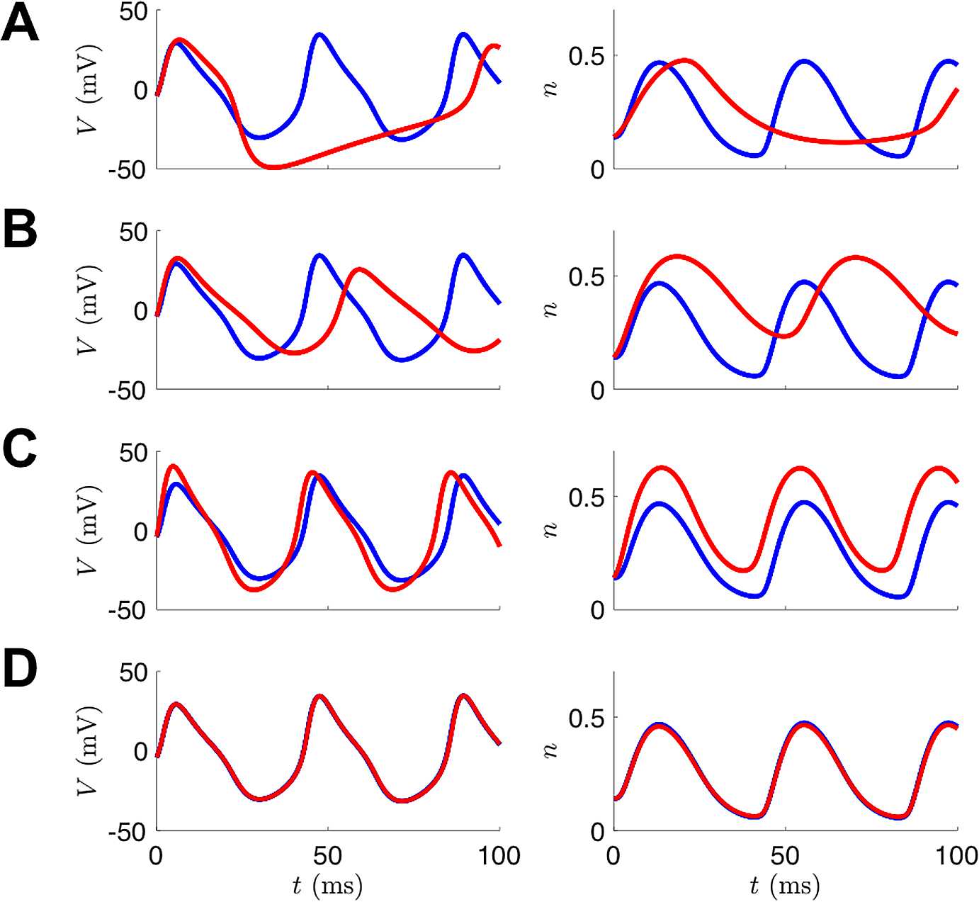
Fig. 10.

Example of 4D-Var assimilation initializing with parameters from the Hopf regime but observational data from the SNIC regime. The blue traces are noiseless versions of the observed voltage data (left column) or the unobserved variable n (right column) from the model that produced the data. The red traces are the result of integrating the model with the estimated parameter sets at various points during the course of the optimization. (A) Initial parameter guesses. (B) Parameter values after 100 iterations. C: Parameter values after 1000 iterations. D: Parameter values after 30,000 iterations (corresponds to t:SNIC/g:HOPF column of Table 3)