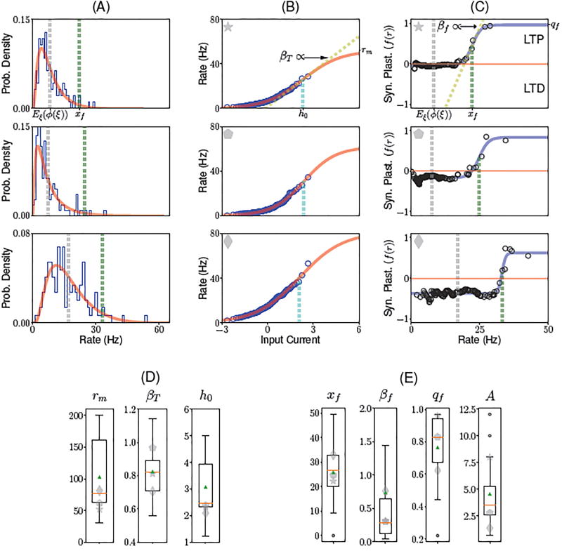
Figure 2.

Inferring transfer function and learning rule from ITC data. (A) Distributions of firing rates in response to novel stimuli, for three different ITC neurons. Blue histogram: histogram of experimentally recorded visual responses. Red: Distribution of firing rates obtained from passing a standard normal distribution through the sigmoidal transfer function shown in B. Gray vertical line: average firing rate. Green vertical line: learning rule threshold x_f (see C). (B) Static transfer function ϕ derived from the distribution of visual responses for novel stimuli (see A), assuming a Gaussian distribution of inputs (see (Lim et al., 2015) and Methods) for the same three neurons shown in A. The data (blue circles) was fitted using a sigmoidal function (red line; see Methods, Eq. (17)), defined by three parameters: the current h₀ that leads to half the maximal firing rate (cyan dashed lines), a slope parameter β_T (dashed yellow line in top plot), and maximal firing rate r_m. (C) Dependence of the synaptic plasticity rule on the postsynaptic firing rate as a function of firing rate (i.e. f(r)). The data (black circles) was fitted with a sigmoidal function (blue line; see Methods, Eq. (22)), defined by three parameters: maximum potentiation q_f; threshold x_f (see green dashed line); and slope parameter β_f (dashed yellow line in top plot). On the right axis is indicated the maximum potentiation of the fit q_f. (D) Boxplot for the fitted parameters r_m, β_T and h₀ of the transfer function. (E) Boxplot for the fitted parameters x_f, β_f, q_f of the dependence of the synaptic plasticity rule on the postsynaptic firing rate, and A, the learning rate. The red line and green triangle indicate the median and the mean of the fitted parameters, respectively. Gray symbols indicate the parameters of the three neurons shown in A,B,C.