Fig. 4.

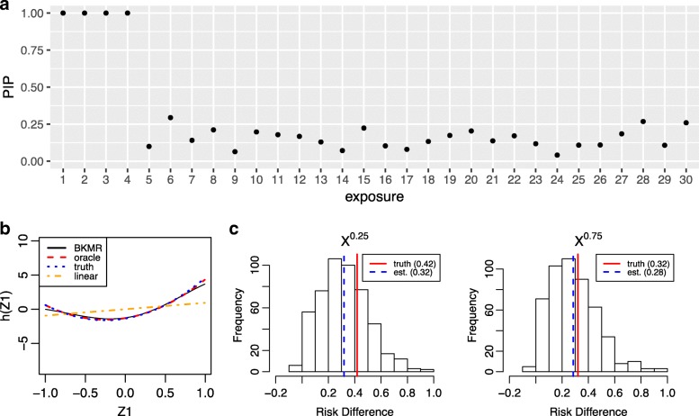
Example output from fitting probit Bayesian kernel machine regression to simulated data. a Posterior inclusion probabilities (PIPs) provide a measure of variable importance ranging from 0 to 1. Exposures 1–4 were included in h in the true data-generating model. b Univariate exposure-response function of z₁ estimated from BKMR, in comparison to a probit generalized linear model (GLM) assuming linear terms of each of the exposure variables (“linear”), a probit GLM that uses the correct model form (“oracle”), and the true exposure-response function (“truth”). Under probit regression, h may be interpreted as the relationship between the exposure variables and an underlying, continuous latent outcome (e.g., a continuous marker of underlying health status for a binary health outcome). c Posterior distribution of the risk difference comparing the probability of the binary outcome when exposure 2 is at its 75th percentile versus its 50th percentile, for all of the exposures fixed at their median value, and for the single confounder x fixed at its 25th or 75th percentile (left and right panels, respectively), along with the posterior mean estimate (“est”) and the true risk difference (“truth”)