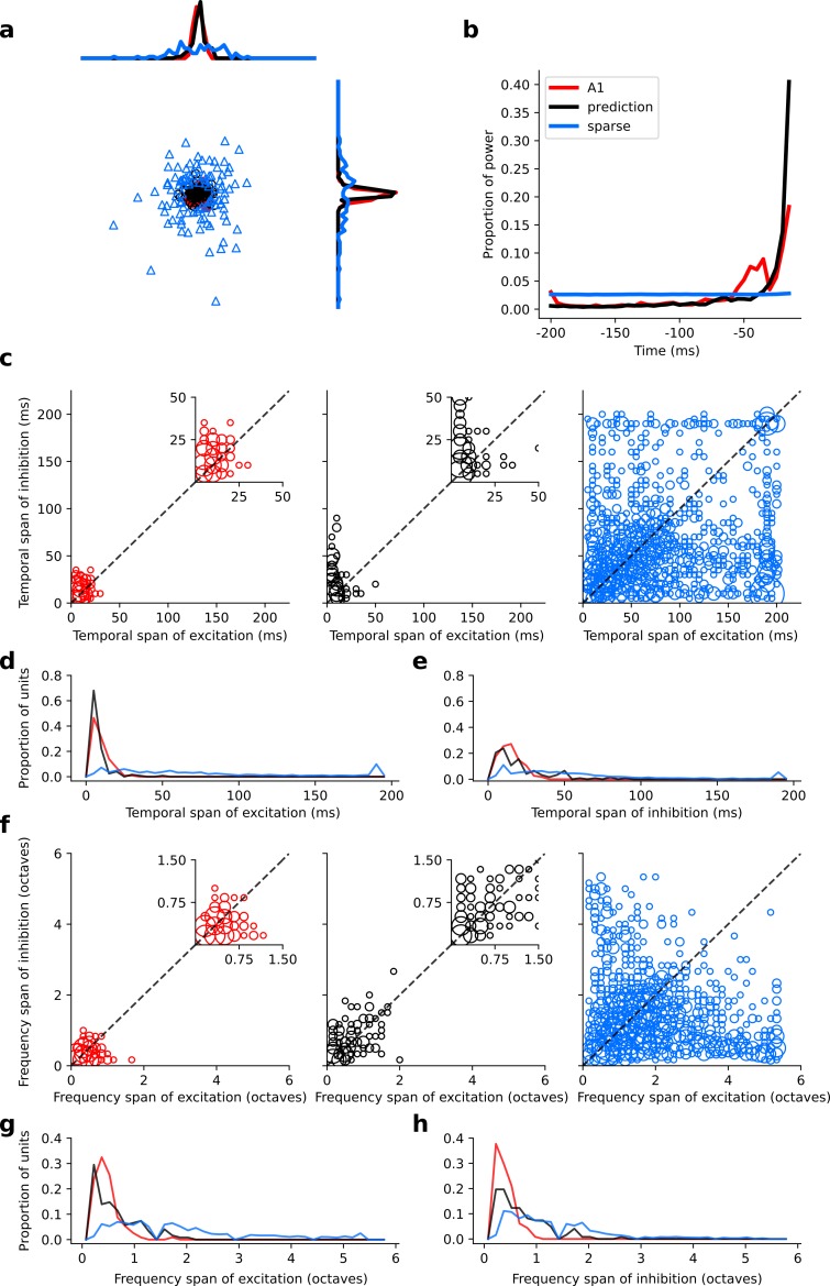
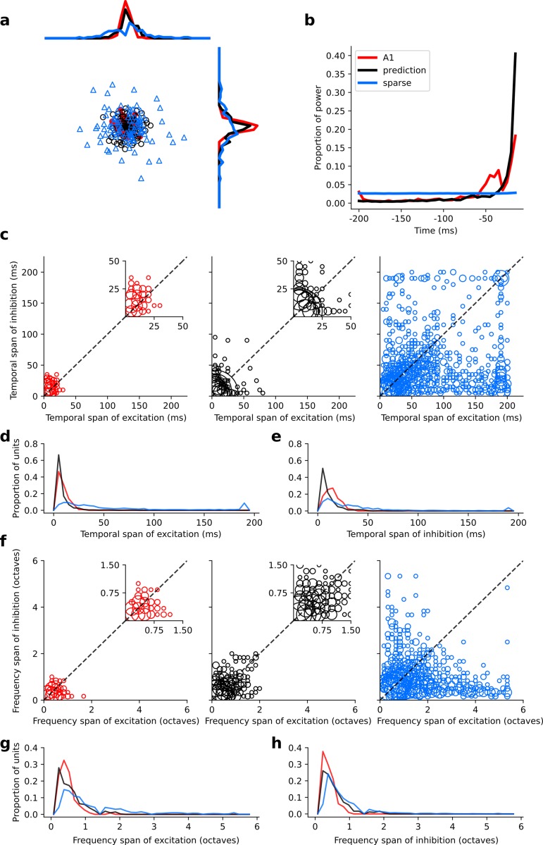
Figure 6. Population measures for real A1, temporal prediction model and sparse coding model auditory spectrotemporal RFs.
The population measures are taken from the RFs shown in Figures 3–5. (a), Each point represents a single RF (with 32 frequency and 38 time steps) which has been embedded in a 2-dimensional space using Multi-Dimensional Scaling (MDS). Red circles - real A1 neurons, black circles – temporal prediction model units, blue triangles – sparse coding model units. Colour scheme applies to all subsequent panels. (b), Proportion of power contained in each time step of the RF, taken as an average across the population of units. (c), Temporal span of excitatory subfields versus that of inhibitory subfields, for real neurons and temporal prediction and sparse coding model units. The area of each circle is proportional to the number of occurrences at that point. The inset plots, which zoom in on the distribution use a smaller constant of proportionality for the circles to make the distributions clearer. (d), Distribution of temporal spans of excitatory subfields, taken by summing along the x-axis in (c). (e), Distribution of temporal spans of inhibitory subfields, taken by summing along the y-axis in (c). (f), Frequency span of excitatory subfields versus that of inhibitory subfields, for real neurons and temporal prediction and sparse coding model units. (g), Distribution of frequency spans of excitatory subfields, taken by summing along the x-axis in (f). (h), Distribution of frequency spans of inhibitory subfields, taken by summing along the y-axis in (f). Figure 6—figure supplement 1 shows the same analysis for the temporal prediction model and sparse coding model trained on auditory inputs without added noise.


