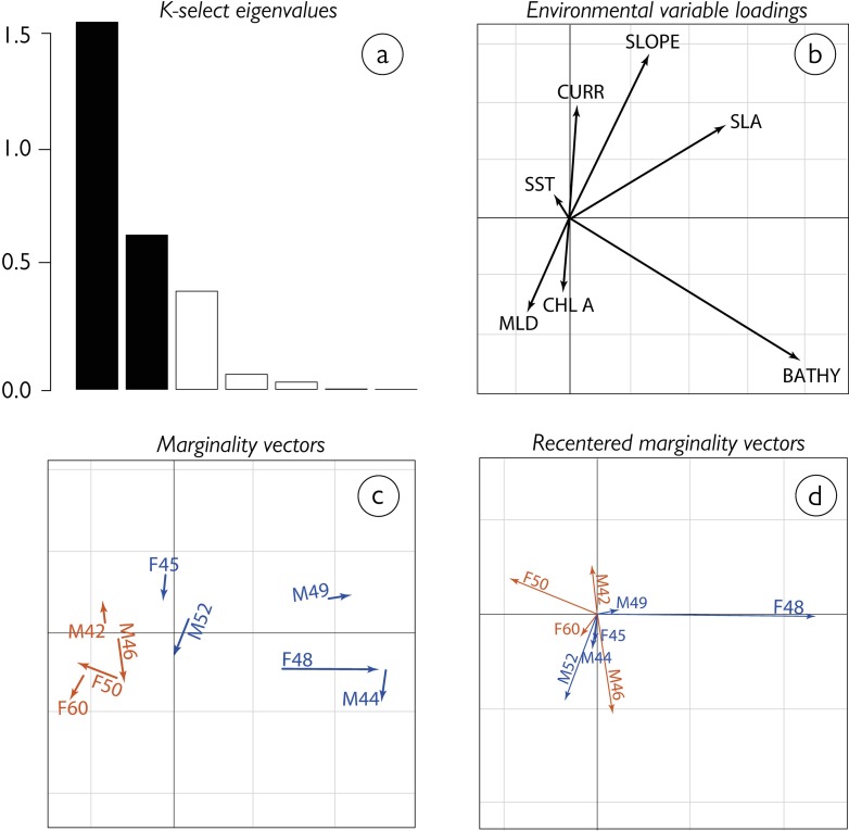
Fig 5. Habitat selection of nine Tawaki during two weeks centred around their trip reversal date, i.e. at their pre-moult journey destinations.

(A) Bar chart of the K-select eigenvalues measuring the mean marginality explained by each factorial axis. (B) Loadings of environmental variables on the first two factorial axes–surface current velocity (CURR), seafloor sloping gradient (SLOPE), Sea Level Anomaly (SLA), water depth (BATHY), Chlorophyll a concentration (CHLA A), Mixed Layer Depth (MLD) and Sea Surface Temperature (SST). Note that water depth (BATHY) is measured as negative integers so that its loading is reversed in comparison with all other variables. (C) Marginality vectors of the individual penguins, where the base of the arrows indicates the mean composition of the habitat at the journey destination, while arrow length and direction correspond to the mean characteristics of the habitat the individuals moved towards during that time. (D) Recentered projection of the marginality vectors such that habitat availability is the same for all animals.