Figure 1.

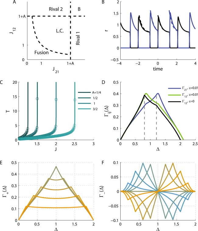
Neuronal dynamics. (A) The phase diagram. The regions of different types of solutions for the neuronal dynamics are depicted in the (quarter of the) plane of (non-negative) J₂₁ and J₁₂. (B). The limit cycle solution. The firing rate of populations 1 and 2 are plotted in black and blue, respectively, as a function of time (measured in units of τ_a) in the anti-phase oscillatory solution with T₁ = 1.2 and T₂ = 0.8, yielding J₂₁ ≈ 2.36 and J₁₂ ≈ 1.87 (see Eq. (43)). In this specific example we used I = 2, A = 2, the solid lines show the solution for $ϵ=0.01$ and the dashed depict the solution in the limit of $ϵ\to 0$. (C) The oscillation period along the diagonal. The oscillation period on the diagonal is shown as a function of the reciprocal inhibition strength for different values of the adaptation strength, A = 0.25, 0.5, 1, 1.5 from left to right. Solid lines show the analytical relation of Eq. (44) in the $ϵ\to 0$ limit. The circles depict the $ϵ=0.01$ case. (D) The cross-correlation function. The neuronal cross-correlations Γ₁₂ (green and black) and Γ₂₁ (blue) are plotted as a function of the time difference, Δ (measured in units of the adaptation time constant τ_a). The black line depicts the correlations in the $ϵ\to 0$ limit, whereas the green and blue lines show the $ϵ=0.01$ case. Parameters were identical to B. For the $ϵ=0.01$ case the correlations were evaluated from the numerical solution for the dynamics. (E) The ‘mean cross-correlation’ function. The mean correlation, Γ₊, in the limit of $ϵ\to 0$, (see subsection Calculation of the cross-correlation function in Methods) is plotted as a function of Δ for T = 2 and different values of the T₁ = T[0.1, 0.2, … 0.9] shown by color. Note that the plots for T₁ = x and T₁ = T − x overlap. (F) The ‘difference cross-correlation’. The difference in the cross-correlation, Γ₋, in the limit of $ϵ\to 0$, is plotted as a function of Δ for T = 2 and different values of the T₁ = T × {0.1, 0.2, … 0.9} shown by color from yellow (T₁ = 0.1T) to blue (T₁ = 0.9T). In E and F A = 2 and I = 2 were used.