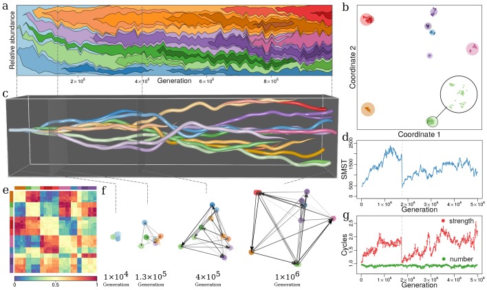
Figure 3. Evolutionary dynamics of a community driven by competitive interactions, with trade-off between fecundity and competitive abilities ($\delta =0.5$, $\lambda =300$, $\mu =0.001$, $m=0.02$, $N_s={10}^5$).

(a) Species’ frequencies over time (Muller plot): one color per species, vertical width of each colored region is the relative abundance of respective species. Frequencies are recorded every ${10}^4$ generations over ${10}^6$ generations. The plot was produced with R-package MullerPlot (Farahpour et al., 2016). (b) Distribution over trait space: Snapshot of distribution of strains and species in trait space after ${10}^6$ generations. By using classical multidimensional scaling the multidimensional trait space is reduced to two dimensions that explain most of the variance in trait space (see Appendix 1, Classical multi-dimensional scaling (CMDS)). Points and discs are strains and species, respectively (see Appendix 1, Species and strains). Magnified disc in lower right corner shows strains in the light green species disc. Discs diameter are proportional to the total abundance of corresponding species, i.e. the sum of relative abundances of all strains that belong to that species. In this snapshot $N_{st}=660$ and $N_{sp}=10$. (c) Evolutionary dynamics in trait space: Snapshots as in panel (b), but concatenated for all times (horizontal axis), from the monomorphic first generation to generation ${10}^6$. Figure 3—video 1 shows this evolutionary dynamics over time. (d) Functional diversity over time (see Appendix 1, Diversity indexes and parameters of dynamics) measured by the size of minimum spanning tree (SMST) in interaction trait space (see Appendix 1, SMST and distribution of species and strains in trait space). At $1.75\times {10}^6$ generations diversity collapses with all species but one going extinct (vertical dashed line) (Appendix 1, Collapses of diversity). (e) Heatmap of interaction matrix $I$ for generation ${10}^6$. Row and column order reflects species consistent with panel (b) and indicated by color bars along top and left. Colors inside heat map represent values of interaction terms (color-key along bottom). (f) Evolution of dominance network: several snapshots from panel (c) with dominance edges, $W_{ij}^{sp}$ between species (colored discs). (g) Numbers and mean strength of cycles over time in green and red, respectively. The strength of a cycle is defined by its weakest edge. Number and mean strength are given in units of number and mean strength of equivalent random networks, respectively (Appendix 1, Intransitive dominance cycles). Right ends in (a) and (c) correspond to generation panel (b) and (e). Colors of species are the same in panels (a), (b), (c), (e) and (f). Note that time scales differ between panels (a), (c) and (d), (g).

Figure 3—video 1. Divergent eco-evolutionary dynamics in interaction trait space.

Download video file ^{(253.5KB, mp4)}

DOI: 10.7554/eLife.36273.006