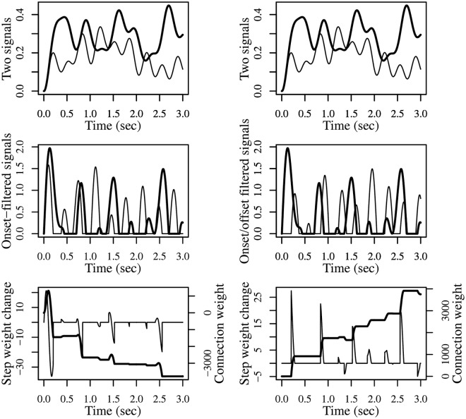
Fig 4. Different filters applied to the same neural signals detect different desired changes and produce different events on which the G-DHL rules can work.

The two columns of graphs refer to two different simulations. The simulations start from the same neural signals (top graphs) but use different filters (middle graphs) leading to a different synaptic update even if the same DHL rule is applied (bottom graphs). Top graphs: each graph represents two signals u₁ and u₂ each generated as an average of 4 cosine functions having random frequency (uniformly drawn in [0.1, 3]) and random amplitude (each cosine function was first scaled to (0, 1) and then multiplied by a random value uniformly drawn in (0, 1)). Middle graphs: events resulting from the filters ${\left[{\dot{u}}_1\right]}^{+}$ and ${\left[{\dot{u}}_2\right]}^{+}$ (left) and from the filters ${\left[{\dot{u}}_1\right]}^{+}$ and ${\left[{\dot{u}}_2\right]}^{-}$ (right; these filters should not be confused with the analogous filters used within the G-DHL rule). Bottom graphs: step-by-step update of the connection weight (thin curve), and its level (bold curve), obtained in the two simulations by applying the Porr-Wörgötter DHL rule to the filtered signals.