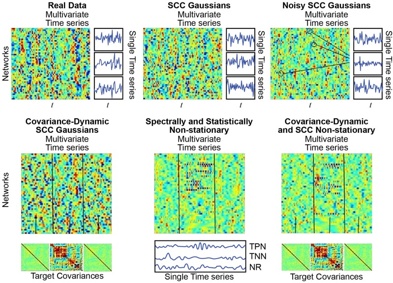
Figure 7.

(Top Left) Real Data: Multivariate timeseries consisting of network timecourses from an actual rs-fMRI subject (Allen et al., 2014) (3 single network examples displayed immediately to the right); (Top Middle) SCC Gaussians: Multivariate timeseries of SCC Gaussians modeled on mean spectral content and mean mutual covariance of empirical network timecourses from the study shown at the top left. (Top Right) Noisy SCC Gaussians: The same as SCC Gaussians but with between 3 and 15 high-amplitude, high-frequency “spikes” interspersed, examples circled. No more than one spike is inserted in any individual timecourse and at most 15 of the 47 timecourses contain spikes. (Bottom Left) Covariance-Dynamic SCC Gaussians: This regime starts like the SCC Gaussians, in that the timeseries are spectrally matched to the mean spectral content of the target empirical dataset. However, the next stage involves covariance matching the middle interval to the mean mutual covariance of the empirical networks, while the first and final intervals are matched to a very weakly connected covariance structure. (Bottom Middle) Spectrally and Statistically Non-stationary: This regime also starts like the SCC Gaussians, in that the timeseries are spectrally and covariance matched to the mean spectral content and covariance structure of the target empirical dataset. Here though there is a middle window in which a subset of TPNs exhibits high-amplitude, high frequency behavior, a subset of TNNs exhibits low-amplitude, low-frequency behavior and most networks are NR to the stimulus. (Bottom Right) Covariance Dynamic and SS Non-stationary: This regime starts like the Covariance Dynamic SCC Gaussians, then a subset of TPNs and TNNs are chosen to respond in the same way as in the Spectrally and Statistically Non-stationary regime.