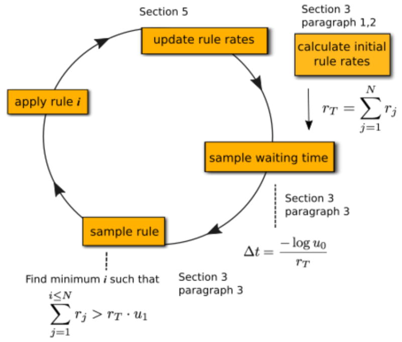
Fig. 1.

A simple graphical depiction of a generalization of Gillespie’s direct method, where N is the total number of rules. Sections describing the relevant steps are labeled in the figure. After initially computing the rates for every rule, each iteration of the simulation loop requires generating two pseudorandom numbers u₀ and u₁ on the interval [0,1). The waiting time until the next event, Δt, is calculated from the first random number and it is inversely proportional to the total rate of the rules in the system: r_T. Then rule i is sampled, where i is the smallest number such that the cumulative rate of rules 0 through i is greater than the product of the second random number and the total rate, r_T. After both the next event time and rule (i.e., the type of reaction) are sampled, the rule is applied to a specific set of molecules from among all molecules that qualify as reactants, and the rates are updated based on the change of the system.