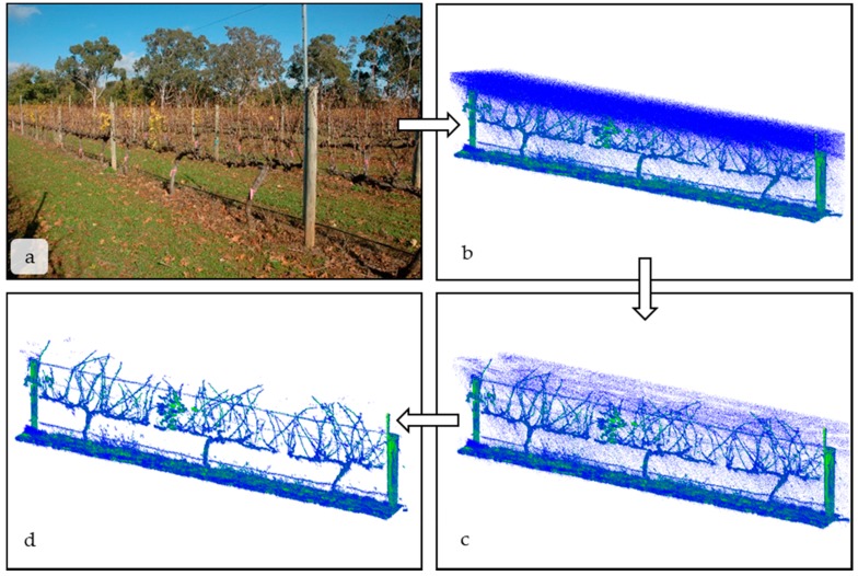
Figure 2.

Following the arrows clockwise from panel (a–d), this figure depicts the workflow used to process scans before computational analysis. (a) depicts a single panel of vines in May 2015 after nearly complete senescence; (b) shows the raw LiDAR scan of the panel before any erroneous points are removed using an intensity filter. Less reflective, low intensity returns are blue (e.g., green grass) and more reflective, high intensity points (e.g., senesced leaves, leaf litter) are green and yellow; (c) shows the LiDAR scan after removal of low intensity points; (d) is the LiDAR scan after a nearest neighbor filter is applied to remove any outliers. All scans are visualized and processed using the open source program CloudCompare.