Abstract
Spectral computed tomography (CT) has been a promising technique in research and clinic because of its ability to produce improved energy resolution images with narrow energy bins. However, the narrow energy bin image is often affected by serious quantum noise because of the limited number of photons used in the corresponding energy bin. To address this problem, we present an iterative reconstruction method for spectral CT using nonlocal low-rank and sparse matrix decomposition (NLSMD), which exploits the self-similarity of patches that are collected in multi-energy images. Specifically, each set of patches can be decomposed into a low-rank component and a sparse component, and the low-rank component represents the stationary background over different energy bins, while the sparse component represents the rest of different spectral features in individual energy bins. Subsequently, an effective alternating optimization algorithm was developed to minimize the associated objective function. To validate and evaluate the NLSMD method, qualitative and quantitative studies were conducted by using simulated and real spectral CT data. Experimental results show that the NLSMD method improves spectral CT images in terms of noise reduction, artifacts suppression and resolution preservation.
Keywords: spectral CT, image reconstruction, nonlocal low-rank and sparse matrix decomposition, photon counting detector
1. Introduction
Spectral CT, or multi-energy CT, has attracted increasing attention in recent years because of its ability in discriminating different materials. Dual energy CT is a simple realization of spectral CT that differentiates material by using two distinct beam energies, including a dual x-ray source (Graser et al., 2009), a fast kVp switching (Zou and Silver, 2008), a dual layer detector (Kim et al., 2015a), etc. Another approach to realize spectral CT is to use a photon counting detector (PCD) with energy discrimination capability (Taguchi and Iwanczyk, 2013). In spectral CT with PCD, polychromatic x-ray photons can be sorted and counted in different energy bins according to the preset energy thresholds (Taguchi and Iwanczyk, 2013). As a result, multiple projection data with different energy information can be generated from a single scan without additional exposure. The selection of energy bins has a critical impact on noise and energy resolution of the multi-energy images (Leng et al., 2011). Generally, the x-ray spectrum need to be divided into more energy bins for higher energy resolution. However, increasing the number of energy bins will lead to few available photons in each energy bin. According to the Poisson noise modeling, this implies higher noise level in the projection data and the image quality of spectral CT reconstructed using the filter back-projection (FBP) algorithm will be greatly degraded (Leng et al., 2011; Yu et al., 2016; Zeng et al., 2016b; Zhang et al., 2016; Li et al., 2015; Niu et al., 2016). Therefore, noise reduction in narrow energy bin image is very important for PCD-based spectral CT reconstruction.
Over the years, the sparsity-regularized methods (e.g., total variation (TV) (Sidky and Pan, 2008; Chen et al., 2008; Liu et al., 2012; Tian et al., 2011; Zhang et al., 2017a), structure tensor TV (Lefkimmiatis et al., 2015), total generalized variation (Niu et al., 2014), and tight frame (Jia et al., 2011)) have been widely explored and have been instrumental for CT reconstruction. In each energy bin, the image can be independently reconstructed using these sparsity-regularized methods. For example, a statistical interior tomography method was employed to reconstruct each energy bin image with TV regularization (Xu et al., 2012a). A structure tensor TV regularization was incorporated into a penalized weighted least-squares (PWLS) principle for spectral CT reconstruction (Zeng et al., 2016a). An iterative reconstruction method based on tight frame was proposed for spectral breast CT using fewer projections while achieving greater image quality (Zhao et al., 2013). However, all the aforementioned methods only consider each energy bin individually and do not use the correlation between different energy bins. The images in different energy bins are highly correlated, as all projection data are obtained from the same object. The low-rank prior information is an effective constraint to exploit the correlation between different energy bins, and the nuclear norm regularization can be introduced to improve the performance of spectral CT reconstruction. Semerci et al. proposed a tensor-based nuclear norm regularization for spectral CT reconstruction, which models the multiple sets of images in different energy bin as a three-way tensor (Semerci et al., 2014). Rigie and La Rivière presented an iterative reconstruction method for jointly reconstructing spectral CT using the total nuclear variation, which couples different energy bins by encouraging the gradient of the corresponding images to point in one direction (Rigie and La Riviere, 2015). Gao et al. developed a PRISM (prior rank, intensity and sparsity model) method for spectral CT reconstruction, which utilizes the low-rank and sparse matrix decomposition to exploit the correlation between the different energy bin images (Gao et al., 2011). Li et al. extended multi-energy images from a matrix form to a tensor form to improve the PRISM method (Li et al., 2014). In addition, Kim et al. developed a patch-based low-rank regularization for sparse-view spectral CT reconstruction (Kim et al., 2015b).
Recently, nonlocal self-similarity using similar patches has been exploited to reduce noise in image reconstruction (Xu et al., 2012b; Zhao et al., 2012; Zhang et al., 2017b; Bian et al., 2013; Ma et al., 2012b; Zhang et al., 2014b; Zhang et al., 2015; Zhang et al., 2014a; Kim et al., 2015b). For example, a patch-based dictionary learning was incorporated into a statistical iterative reconstruction for low-dose CT (Xu et al., 2012b). Later, a patch-based dual-dictionary learning was proposed for spectral CT reconstruction, in which two dictionaries from different images was used (Zhao et al., 2012). More recently, the dictionary learning was extended from a vector form to a tensor form for spectral CT reconstruction (Zhang et al., 2017b). In addition, Zhang et al. explored the nonlocal mean-based regularization under PWLS principle for low-dose CT reconstruction (Zhang et al., 2014b; Zhang et al., 2015). Incorporating a high quality image into reconstruction, Zhang et al. proposed a prior image induced nonlocal regularization for statistical iterative reconstruction (Zhang et al., 2014a).
To incorporate the correlation in multi-energy images, we propose a nonlocal low-rank and sparse matrix decomposition (NLSMD) for spectral CT reconstruction. We group the similar patches in multi-energy images to form a matrix, then decompose it into the summation of a sparse matrix and a low-rank matrix. The sparse matrix represents the different intensity feature that is sparse under a sparse transform, while the low-rank matrix represents the rest of stationary background that is low-rank. The novelty of the NLSMD method is threefold. First, the proposed method works as a local low-rank and sparse matrix decomposition for similar patches, and reduce noise artifacts while preserving detail features such as edge and structure information. Second, there are usually less than two materials inside the small patches, which means that a relative low-rank structure. Third, an alternating minimization algorithm was adopted to solve the associated objection function. Qualitative and quantitative evaluation conducted with simulated and real PCD data clearly demonstrated that NLSMD method outperforms the existing robust principal component analysis (RPCA) method in terms of noise reduction, artifacts suppression and resolution preservation.
The remaining part of this paper is organized as follows. Section 2 develops the NLSMD based spectral CT reconstruction method. We also describe the experimental setup and quantitative evaluation metrics. Section 3 reports simulated and real PCD data experiments and results. Finally, section 4 gives the discussion and conclusion.
2. Materials and methods
2.1. Spectral CT imaging
In spectral CT with PCD, several projection data were acquired from polychromatic x-ray spectrum. The projection of each energy bin can be approximately formulated as a series of linear equations as follows:
| (1) |
where A is the system or projection matrix with the size of M × N, yk=(yk,1, yk,2, ⋯ yk,M) is the projection data of the k th energy bin, xk= (xk,1, xk,2, ⋯, xk,N) denotes the k th energy bin image, and K is the number of energy bins. We define data sets of and , where T denotes the transpose operator. Using above notations, the Eq. (1) can be rewritten as Y = AX.
To solve the problem (1), the cost function with a regularization/prior term R(X) is used as follows:
| (2) |
where ‖·‖F denotes the Frobenious norm, β > 0 is a smoothing or penalty parameter that controls the relative contribution from the data fidelity term and regularization/prior term.
2.2. NLSMD for spectral CT reconstruction
In this study, we use the nonlocal low-rank and sparse matrix decomposition to exploit the self-similarity of the multi-energy images. The similar small patches are collected at the same position in multi-energy images, and are grouped into one matrix
| (3) |
where {Rpxk}(p= 1, 2, ⋯, P;k= 1,2, ⋯, K) is a patch extraction operator which is defined as a mapping form ℝN to ℝB, p and k are the indexes for a specific p patch in the kth energy bin image, B is the number of pixels within a patch of size , and P is the number of patches. Since these patches have similar structures, thus they should locate in a low-dimension subspace. Motived by this observation, we model the matrix Vp as: Vp = Lp + Sp, where Lp denotes a low-rank matrix, Sp denotes a sparse matrix. The matrices Lp and Sp can be recovered by solving the following minimization problem:
| (4) |
where ‖·‖* is the nuclear norm, ‖·‖1 is the ℓ1 norm, λ > 0 is a penalty parameter that balances the nuclear norm term and the ℓ1 norm term, TS denotes some proper transform so that the matrix Sp becomes more sparser. Instead of minimizing the constrained optimization problem (4), we rewrite it as the following unconstrained minimization problem:
| (5) |
Here TS can be any sparsifying transform, for simplicity, TS is chosen to be discrete gradient transform.
Using the above NLSMD, we propose the following objective function for spectral CT reconstruction:
| (6) |
where ∇ represents the discrete gradient transform, and the value of λ is set as suggested by (Candès et al., 2011):
| (7) |
where n1 and n2 are the number of rows and columns of the matrix Vp.
2.3. Optimization algorithm
To solve the proposed objective function in Eq. (6), we alternatively minimize X, Lp and Sp as follows:
| (8) |
| (9) |
| (10) |
2.3.1. Minimization with respect to (Lp, Sp)
Note that the sub-problem (9) is independent to the data fidelity term, and it can be minimized patch by patch. Therefore, for a given , the Eq. (9) can be solved by alternatively minimizing Lp and Sp, respectively. For a fixed Sp, Lp can be solved by minimizing
| (11) |
The solution of (11) is given by the singular value thresholding algorithm (Cai et al., 2010):
| (12) |
where σi, ui, and vi are the singular values and vectors of . For a fixed Lp, Sp is solved by minimizing
| (13) |
The solution of (13) can be obtained using the Chambolle projection algorithm (Chambolle, 2004). In the scheme of Chambolle algorithm, we solve the following constrained minimization problem:
| (14) |
where Wi,j is the dual variable at the (i, j) th location, W is the concatenation of all Wi,j, α = λμ, and div is divergence operator. When the minimum W* of the problem (14) is obtained, the solution of (13) can be directly obtained as follows:
| (15) |
The iterative scheme for the W* is given as follows:
| (16) |
where is the lth iteration, τ > 0 is the step size used in the Chambolle projection algorithm. For each outer iteration, the number of Chambolle projection algorithm was fixed to 20.
2.3.2. Minimization with respect to X
Note that each patch is voxel-shifted from a previous patch, and each voxel in the multi-energy images is overlapped B times for the patch grouping. Hence, the inverse transform from the patch to the image domain can be formulated as . With the definition , we have
| (17) |
Consequently, using (17), the solution of (10) can be derived from the following optimal condition
| (18) |
Here, the conjugate gradient (CG) algorithm is used to solve the linear system. Since the linear system is symmetric positive definite, CG algorithm can get an exact solution after a few iterations, e.g. 5 iterations.
2.4. Experimental data
2.4.1. Simulation data
Five monochromatic images (60, 70, 80, 90, and 100 keV) acquired by a GE Discovery CT750 CT scanner were used to simulate the multi-energy projection data. The x-ray spectrum of 140 kV (Fig. 1) was generated by the TASMICS method (Hernandez and Boone, 2014). Poisson noise is superimposed to the measurement by assuming 1.0 × 10⁵ photons emitted from the x-ray source. The emitted photons were distributed to each energy bin with the weights calculated from the x-ray spectrum in Fig. 1. Using the previously developed simulation method in (Zeng et al., 2016b), the projection data of five energy bins were obtained in a fan-beam CT geometry. The distance from the x-ray source to the detector arrays was 949 mm and the distance from the detector arrays to the rotation center is 408 mm. The number of detector elements is 888 and the space of each detector bin is 1.0 mm. To demonstrate sparse-view spectral CT reconstruction, only 88 projection views of each energy bin were collected over a full scan range.
Figure 1.
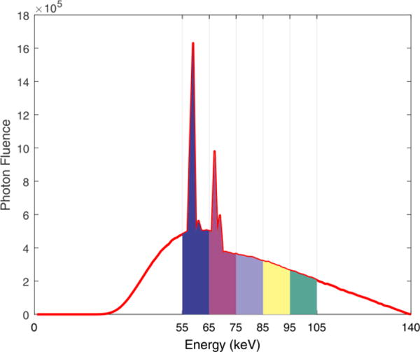
X-ray spectrum of 140 kV with five energy bins.
2.4.2. Ex vivo data
A lamb chop was scanned by MARS spectral CT with the Medipix3RX PCD. The distance from the source to the center of rotation is 131.8 mm and the distance from the detector arrays to the center of rotation is 48 mm. The x-ray tube was set at 50 kV with the current of 120 μA using four energy thresholds (15, 20, 25, and 30 keV). More details about this dataset can be found in (Aamir et al., 2014). To demonstrate sparse-view reconstruction, we extracted 163 projection views from the full-view projection data in each energy bin.
2.5. Performance evaluation
2.5.1. Image reconstruction accuracy
Relative root mean square error (RRMSE) was employed to evaluate image reconstruction accuracy. The definition of RRMSE is as follows:
| (19) |
where x(n) and nref (n) represent the voxel value of reconstructed and reference images at pixel n, respectively, N is the total number of voxels in the image.
2.5.2. Image similarity metric
The structural similarity (SSIM) (Zhou et al., 2004) is used to evaluate the similarity between the reconstructed and reference images. Given a region of interest (ROI), the mean, variance and covariance in the ROI is defined as follows:
| (20) |
| (21) |
| (22) |
where x(q) denotes the voxel value of the reconstructed image and xref(q) denotes the voxel value of the reference image in the ROI, Q is the total number of voxels in the ROI. The SSIM can be calculated as follows:
| (23) |
where c1and c2 are two constants.
2.5.3. Noise-resolution tradeoff
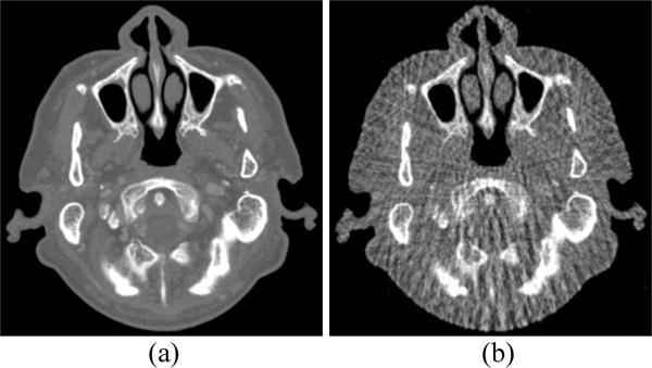
To evaluate the resolution of the reconstructed image, the noise-resolution tradeoff was studied. The resolution is analyzed using the edge spread function (ESF) along the red line in Fig. 4(a). We assume that the standard deviation (SD) of the broadening Gaussian kernel is δ, and the ESF can be characterized by an error function (ER) parametrized by δ. The parameter δ is calculated by fitting the profile along the red line to an ER, and the full-width at half-maximum of the broadening Gaussian function is denoted as 2.35δ, that is, the resolution of the reconstructed image. The noise of the reconstructed image is quantified by the SD of a uniform region of size 20 × 20 in the background region as indicated by the pink square in Fig. 4(a). By changing the penalty parameter μ for NLSMD method, we obtained the noise-resolution tradeoff curve.
Figure 4.
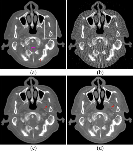
Spectral CT images at 70 keV energy bin: (a) Phantom; (b) FBP image reconstructed from 88 projection views; (c) RPCA image reconstructed from 88 projection views; (d) NLSMD image reconstruction from 88 projection view.
2.5.4. Material decomposition
In the image-domain material decomposition, the linear attenuation coefficient of a CT image can be approximately expressed as the linear combination of two basis materials (Szczykutowicz and Chen, 2010), that is,
| (24) |
where xH/L denotes the high/low energy bin image, xij is the linear attenuation coefficient of basis material i (i= 1 or 2) at the energy bin j (j= H or L), and f1 and f2 represent the material decomposition images. Using the basis materials and the images at high (100 keV) and low (60 keV) energy bins, the material decomposition images can be obtained as follows:
| (25) |
2.5.5. Comparison method
The performance of the NLSMD method was validated and evaluated by comparing it with the robust principal component analysis (RPCA) method. The RPCA method for spectral CT reconstruction can be formulated as follows:
| (26) |
where XL and XS are the low-rank component and sparse component of X, respectively, μ > 0 is penalty parameter, λ is set as similar as Eq. (7). The parameter μ of the RPCA method was chosen manually to perform the best reconstruction result with minimal RRMSE value.
3. Results
3.1. Simulation study
3.1.1. Selection of the parameters in NLSMD method
There are two parameters to be determined in NLSMD method, that is, the patch size and penalty parameter μ. The accuracy of NLSMD reconstruction at 70 keV energy bin is quantified by the RRMSE shown on Fig. 2. For a fixed patch size, the RRMSE of the reconstructed image with various penalty parameters is shown in Fig. 3(a). It was found that the value of RRMSE initially decreases with the increase of μ, and thus, the reconstructed image retains some noise and artifacts. However, when μ > 10−5 the RRMSE is increased, the reconstructed image is overly smooth, which causes a loss in edges and fine structures. Thus, the optimal penalty parameter μ with the minimal RRMSE was used in this study. Meantime, for a fixed penalty parameter μ, the RRMSE of the reconstructed results for different patch sizes is shown in Fig. 3(b). Indeed, the value of RRMSE is lowest for the patch of size 6 × 6. In practice, the optimal patch size may change with reconstruction dimensions, but the patch size is set to 6 × 6 for consistency and fairness.
Figure 2.
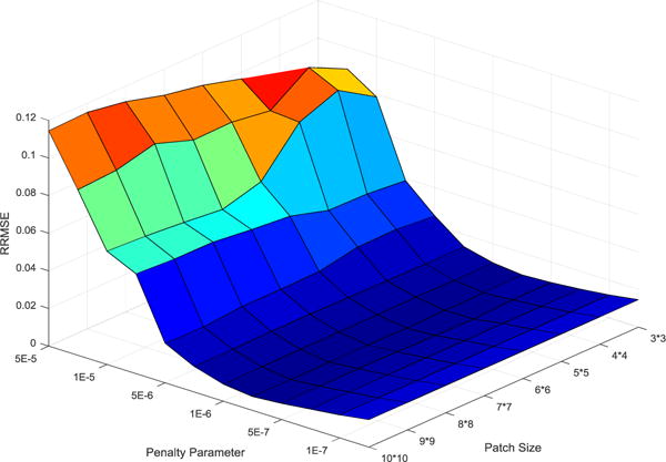
Surface plot of the RRMSE as a function of the patch size and the penalty parameter μ.
Figure 3.
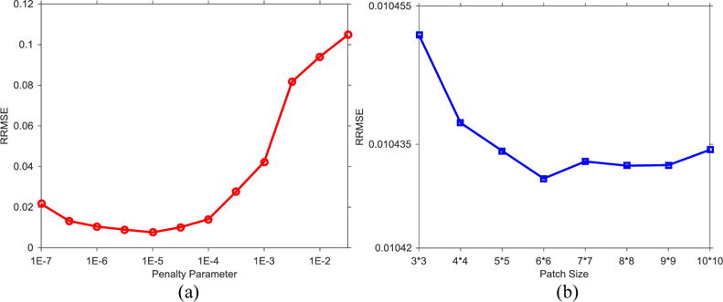
Image reconstruction accuracy of NLSMD method with respect to different penalty parameters and patch sizes: (a) penalty parameter; (b) patch size.
3.1.2. Visual evaluation
The spectral CT images at 70 and 90 keV energy bins are shown in Figs. 4 and 5, respectively. The phantom images are depicted in Figs. 4(a) and 5(a). The FBP results reconstructed from 88 projection views are illustrated in Figs. 4(b) and 5(b). The RPCA results reconstructed from 88 projection views are shown in Figs. 4(c) and 5(c). The NLSMD results reconstructed from 88 projection views are displayed in Figs. 4(d) and 5(d). It can be observed that the FPB images contain serious noise and streak artifacts because of few available photons and insufficient angular sampling in narrow energy bin. The noise and streak artifacts have been effectively reduced in RPCA results, however, some streak artifacts still exist around the skull. We confirmed that the presented NLSMD method achieves the best performance in terms of artifacts reduction and structure preservation as indicated by the arrow in Figs. 4 and 5. The profiles of the RPCA and NLSMD results correspond to the blue line in Fig. 4(a) was plotted in Fig. 6. The reconstructed images using RPCA method produce underestimated values whereas NLSMD method can produce better matching results.
Figure 5.
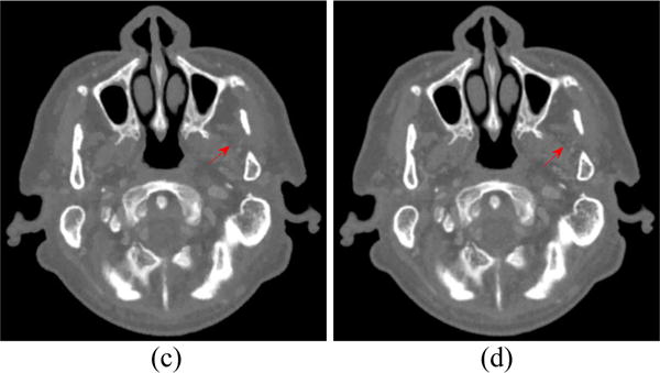
Spectral CT images at 90 keV energy bin: (a) Phantom; (b) FBP image reconstructed from 88 projection views; (c) RPCA image reconstructed from 88 projection views; (d) NLSMD image reconstruction from 88 projection view.
Figure 6.
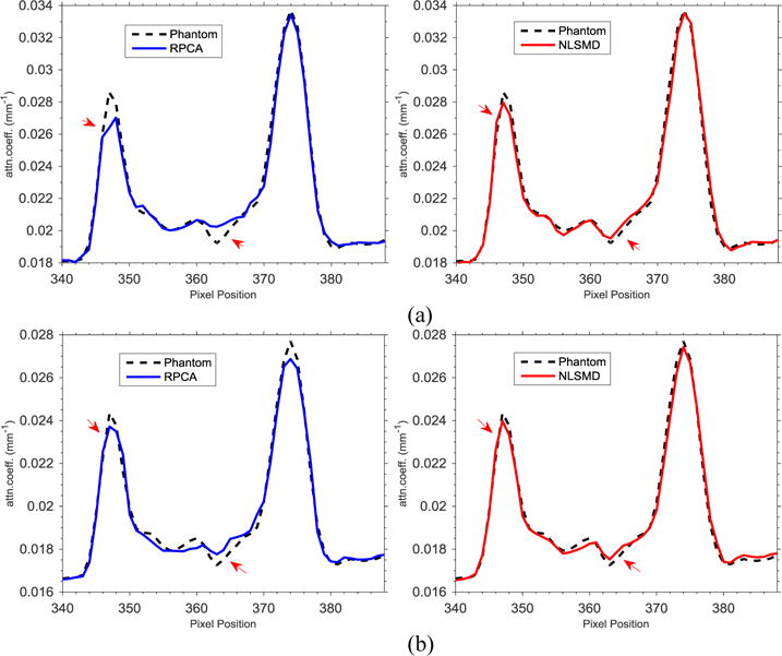
Horizon profiles that correspond to the blue line in Fig. 4(a) of reconstructed images of PRCA and NLSMD methods at different energy bins: (a) 70 keV energy bin; (b) 90 keV energy bin.
3.1.3. SSIM study
To further display the difference between the RPCA and NLSMD results, the zoomed ROI (indicated by the white rectangular in figure 4(a)) is shown in Fig. 7. To quantitative evaluate the performance of NLSMD and RPCA methods with a degree of uncertainty, the experiments were repeated for 10 different instantiations of noise. The corresponding mean and standard deviation of SSIM at each energy bin are illustrated in Fig. 8. There is a 6.14% increase in average SSIM measurement for NLSMD method compared with RPCA method. Moreover, the standard deviations of SSIM measurement from NLSMD method is lower than that from RPCA method, suggesting the robustness of the NLSMD method. We confirmed that the structures in the image reconstructed by NLSMD method are produced with better appearance with less detail loss, especially for the small size structures.
Figure 7.
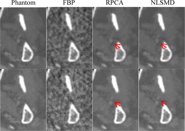
Zoomed-in views of the ROI in images at 70 keV energy bin (first row) and 90 keV energy bin (second row).
Figure 8.
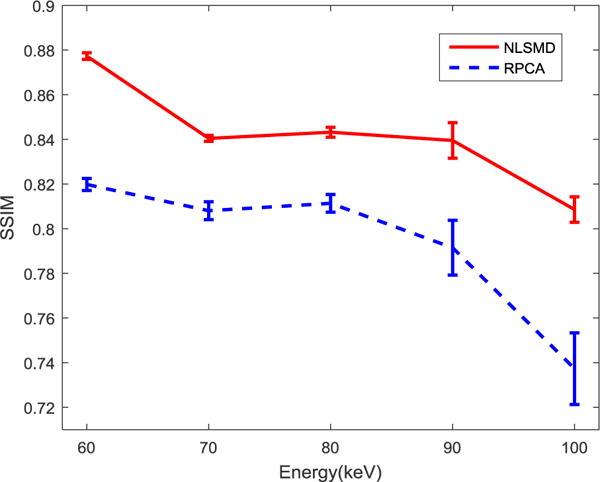
SSIM curves of RPCA and NLSMD results versus the different energy bins. Error bars denote standard deviations of the SSIM distribution for each energy bin with different instantiations of noise.
3.1.4. Noise-resolution tradeoff
The noise-resolution tradeoff curves are displayed for 70 and 90 keV energy bin images in Fig. 9. The noise level of NLSMD results is lower than that of RPCA results with matched spatial resolution. At the 1.8 mm spatial resolution level in two noise-resolution tradeoff curves, the average noise level of NLSMD results is 8.8% lower than that of RPCA results. The results confirm the expected advantages using the nonlocal self-similarity in the spectral CT reconstruction.
Figure 9.
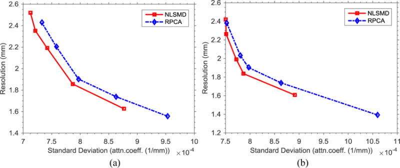
Noise-resolution tradeoff curves of RPCA and NLSMD methods at two different energy levels: (a) 70 keV energy bin; (b) 90 keV energy bin.
3.1.5. Material decomposition
In spectral CT, not only is the image quality important, but accurate material decomposition is also important. The material decomposition images produced using phantom, FPB, RPCA and NLSMD images are shown in Fig. 10. Figs. 10(a) and (e) display the tissue and bone images decomposed using phantom images. Figs. 10(b) and (f) show the tissue and bone images decomposed using FBP images. Figs. 10(c) and (g) represent the tissue and bone images decomposed using RPCA images. Figs. 10(d) and (h) depict the tissue and bone images decomposed using NLSMD images. We can observe that FBP results contain severe noise and artifacts. Although the RPCA results contain less noise and artifacts, many pixels from the boundary of tissue are wrongly categorized as containing bone. Comparing with the material decomposition images from phantom, NLSMD method produces more accurate material decomposition images. To better compare the NLSMD and RPCA methods for material decomposition, the corresponding material decomposition difference images are displayed in Fig. 11. Fig. 11(a) shows the difference image between Fig. 10(a) and Fig. 10(c). Fig. 11(b) displays the difference image between Fig. 10(a) and Fig. 10(d). Fig. 11(c) represents the difference image between Fig. 10(e) and Fig. 10(g). Fig. 11(d) depicts the difference image between Fig. 10(e) and Fig. 10(h). It can be observed that the difference images between NLSMD results and phantom are smaller than that obtained from RPCA results.
Figure 10.
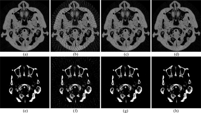
Material decomposition images from different results. Images (a) and (e) display the decomposed tissue and bone images from phantom, respectively. Images (b) and (f) display the decomposed tissue and bone images from FBP results, respectively. Images (c) and (g) display the decomposed tissue and bone images from RPCA results, respectively. Images (d) and (h) display the decomposed tissue and bone images from NLSMD results, respectively.
Figure 11.
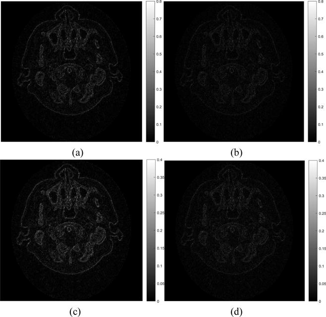
Material decomposition difference images of RPCA and NLSMD results with respect to the phantom. Images (a) and (c) represent the tissue and bone material difference images between RPCA results and phantom, respectively. Images (b) and (d) represent the tissue and bone material difference images between NLSMD results and phantom, respectively.
The zoomed details of material decomposition images are depicted in Fig. 12. It can be clearly observed from the left column in Fig. 12 that many pixels at the tissue gap between bones are incorrectly clarified as containing bone using RPCA method, as indicated by the red arrow. Furthermore, while a few pixels at the nasal cavity are wrongly decomposed as bone using RPCA method, the bone image produced using NLSDM method is correct, as indicated by the red arrow. To quantitatively validate the presented NLSMD method for material decomposition, the SSIM values of FBP, RPCA, and NLSMD results corresponding to Fig. 12 are shown in Fig. 13. These results illustrate that the NLSMD method outperforms RPCA method by incorporating the nonlocal self-similarity between multi-energy images.
Figure 12.
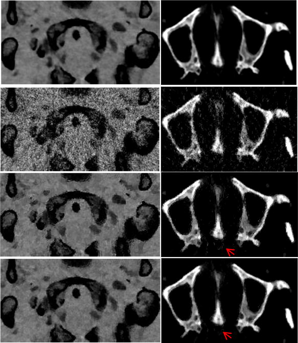
Zoomed details of the decomposed tissue (left column) and bone (right column) images. From top to bottom are phantom, FBP, RPCA, and NLSMD results.
Figure 13.
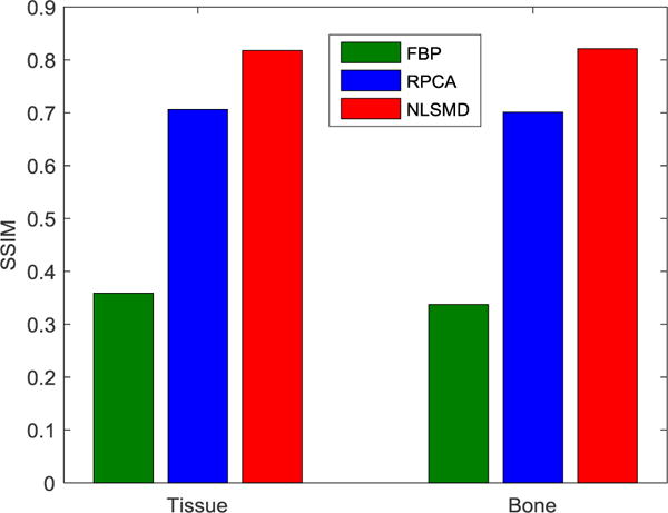
SSIM of the zoomed details of FBP, RPCA, and NLSMD results in Fig. 12.
3.2. Ex vivo data study
The images reconstructed from a real PCD data from MARS scanner are displayed in Fig. 14. The first and second rows of Fig. 14 are the images at 20 keV and 25 keV energy bins, respectively. The FBP images reconstructed from 163-view projection are displayed in Figs. 14(a) and (e). The FBP images reconstructed from full-view projection are represented in Figs. 14(b) and (f). We can observe that high levels of noise exists in FBP images reconstructed from both sparse-view and full-view projection data. The RPCA images reconstructed from 163-view projection are displayed in Figs. 14(c) and (g). The NLSMD images reconstructed from 163-view projection are displayed in Figs. 14(d) and (h). We can observe that the noise in both RPCA and NLSMD results was effectively removed. To further evaluate the performance of RPCA and NLSMD methods, eight ROIs were selected in the meat (the red squares in Fig. 14 (d)) and fat (the blue squares in Fig. 14 (d)) areas to calculate the signal-to-noise ratio (SNR) and contrast-to-noise ratio (CNR) for each reconstruction results. The SNR and CNR were calculated as follows:
| (27) |
| (28) |
Figure 14.
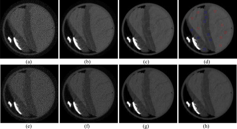
Spectral CT images at 20 keV (first row) and 25 keV (second row) energy bins. Figures (a) and (e) is the FBP results reconstructed from the 163-view projection. Figures (b) and (f) is the FBP results reconstructed from the full-view projection. Figures (c) and (g) is the RPCA results reconstructed from the 163-view projection. Figures (d) and (h) represent the results reconstructed by NLSMD method from the 163-view projection.
The averaged SNR and CNR at four energy bins of RPCA and NLSMD results are depicted in Fig. 15. From this figure, we observe that both the SNR and CNR value of NLSMD results are higher than that of RPCA results.
Figure 15.
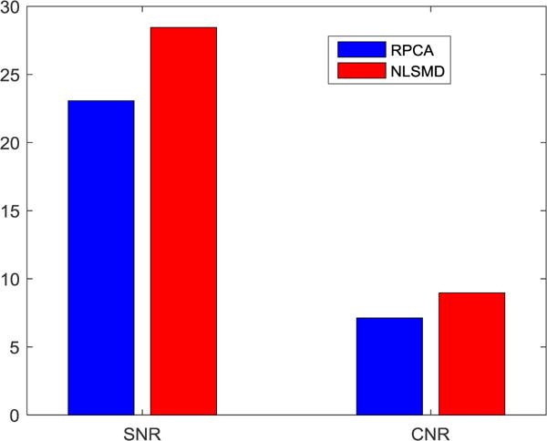
SNR and CNR values of the RPCA and NLSMD results.
4. Discussion and conclusion
In this paper, we proposed an iterative NLSDM method to improve image quality of spectral CT with narrow energy bins. In contrast to existing image reconstruction methods, the proposed NLSMD method utilizes nonlocal low-rank and sparse matrix decomposition to reconstruct spectral CT by explicitly exploring both the sparsity and correlation of different energy bin images. Thus, severe noise and artifacts caused by a limited number of photons and projections in narrow energy bin images can be efficiently suppressed, as depicted by simulated and real spectral datasets studies.
In the simulation study, the proposed NLSMD method outperforms the RPCA method for sparse-view spectral CT reconstruction in terms of reconstruction accuracy and noise-resolution trade-off. For visual inspection, the NLSMD method can produce satisfactory results for spectral CT with narrow energy bins. The profile analysis depicted the further improvement in detailed edge and structure information preservation. The SSIM and noise-resolution tradeoff studies shown that the gain by the use of the NLSMD reconstruction is noticeable compared with RPCA reconstruction. In addition, the NLSMD method was validated and evaluated by the real PCD data from MARS scanner (Aamir et al., 2014). The results show that NLSMD method outperforms the RPCA method on both visual inspection and quantitative evaluation.
Parameter selection plays an important role in iterative CT image reconstruction. There are four main tuning parameters for NLSDM method: the iteration number of the Chambolle projection algorithm, the iteration number of CG algorithm, μ and patch size. In this work, the iteration numbers of the Chambolle projection algorithm and CG algorithm were set to be identical for the simulated and real spectral datasets studies, and satisfactory results were obtained, which shown that these two parameters are suitable for spectral CT reconstruction with narrow energy bins. We validated the performance of NLSMD method by calculating the RRMSE with respect to different values of μ and patch size, as shown in Fig. 2. For the penalty parameter μ, it is the key for the success of NLSMD reconstruction. In the simulation study, we manually selected the parameter μ to obtain the best image quality of spectral CT, as indicated in Fig. 3(a). The optimal value of μ is case dependent, which is determined by the noise level of projection data. Regarding the selection of patch size, we studied the results reconstructed using different patch sizes with a fixed value of μ, and we found that the optimal patch size is 6 × 6, as displayed in Fig. 3(b). In this work, we choose the same penalty parameter for each patch to make it easy to implement in practice. If we minimize Lp and Sp patch by patch with different penalty parameters, the performance of the proposed algorithm could be further improved. However, this will make the optimization problem much more complicated as how to choose an optimal penalty parameter is still an open problem in iterative reconstructions. More effort should be focused on finding an automatic or semi-automatic technique to determine the optimal parameters, which will be an interesting topic in future research.
There are some potential limitations of the proposed NLSMD method in its current version. First, NLSMD method does not take noise statistical properties into account, which plays an important role in CT reconstruction with limited number of photons (Wang et al., 2006; Zhang et al., 2014a; Niu et al., 2017; Wang et al., 2009; Ma et al., 2012a). Incorporating statistical noise modeling into NLSMD reconstruction for spectral CT with narrow energy bins is one of our future research. Second, computational time is a challenge in the practical application of NLSMD method. Nevertheless, the NLSMD reconstruction can be sped up by using dedicated multi-core CPU and graphics processing unit (GPU) hardware in an efficient and parallel fashion (Xu and Mueller, 2005; Li et al., 2005).
Acknowledgments
This work was supported in part by the Cancer Prevention and Research Institute of Texas (RP130109), the American Cancer Society (RSG-13-326-01-CCE), US National Institutes of Health (R01 EB020366), National Natural Science Foundation of China (11701097, 81371544, 61571214, 11661007), Natural Science Foundation of Jiangxi Province (20161BAB212055), Science and Technology Program of Jiangxi Education Committee (GJJ150994 and LDJH12088), NCET Program of the Ministry of Education (NCET-13-0738), National Science and Technology Major Project of the Ministry of Science and Technology of China (No. 2014BAI17B02), and Science and Technology Program of Guangzhou (No. 201510010039). The authors would also like to thank the anonymous referees for their constructive comments and suggestions that greatly improved the quality of the paper.
References
- Aamir R, Chernoglazov A, Bateman CJ, Butler APH, Butler PH, Anderson NG, Bell ST, Panta RK, Healy JL, Mohr JL, Rajendran K, Walsh MF, de Ruiter N, Gieseg SP, Woodfield T, Renaud PF, Brooke L, Abdul-Majid S, Clyne M, Glendenning R, Bones PJ, Billinghurst M, Bartneck C, Mandalika H, Grasset R, Schleich N, Scott N, Nik SJ, Opie A, Janmale T, Tang DN, Kim D, Doesburg RM, Zainon R, Ronaldson JP, Cook NJ, Smithies DJ, Hodge K. MARS spectral molecular imaging of lamb tissue: data collection and image analysis. Journal of Instrumentation. 2014;9:P02005–P. [Google Scholar]
- Bian Z, Ma J, Huang J, Zhang H, Niu S, Feng Q, Liang Z, Chen W. SR-NLM: a sinogram restoration induced non-local means image filtering for low-dose computed tomography. Computerized medical imaging and graphics : the official journal of the Computerized Medical Imaging Society. 2013;37:293–303. doi: 10.1016/j.compmedimag.2013.05.004. [DOI] [PMC free article] [PubMed] [Google Scholar]
- Cai JF, Candes EJ, Shen ZW. A Singular Value Thresholding Algorithm for Matrix Completion. Siam Journal on Optimization. 2010;20:1956–82. [Google Scholar]
- Candès EJ, Li X, Ma Y, Wright J. Robust principal component analysis? Journal of the ACM (JACM) 2011;58:11. [Google Scholar]
- Chambolle A. An algorithm for total variation minimization and applications. Journal of Mathematical Imaging and Vision. 2004;20:89–97. [Google Scholar]
- Chen GH, Tang J, Leng S. Prior image constrained compressed sensing (PICCS): a method to accurately reconstruct dynamic CT images from highly undersampled projection data sets. Medical physics. 2008;35:660–3. doi: 10.1118/1.2836423. [DOI] [PMC free article] [PubMed] [Google Scholar]
- Gao H, Yu H, Osher S, Wang G. Multi-energy CT based on a prior rank, intensity and sparsity model (PRISM) Inverse problems. 2011;27 doi: 10.1088/0266-5611/27/11/115012. [DOI] [PMC free article] [PubMed] [Google Scholar]
- Graser A, Johnson TR, Chandarana H, Macari M. Dual energy CT: preliminary observations and potential clinical applications in the abdomen. European radiology. 2009;19:13–23. doi: 10.1007/s00330-008-1122-7. [DOI] [PubMed] [Google Scholar]
- Hernandez AM, Boone JM. Tungsten anode spectral model using interpolating cubic splines: unfiltered x-ray spectra from 20 kV to 640 kV. Medical physics. 2014;41:042101. doi: 10.1118/1.4866216. [DOI] [PMC free article] [PubMed] [Google Scholar]
- Jia X, Dong B, Lou Y, Jiang SB. GPU-based iterative cone-beam CT reconstruction using tight frame regularization. Physics in medicine and biology. 2011;56:3787–807. doi: 10.1088/0031-9155/56/13/004. [DOI] [PubMed] [Google Scholar]
- Kim DW, Kim HK, Youn H, Yun S, Han JC, Kim J, Kam S, Tanguay J, Cunningham IA. Signal and noise analysis of flat-panel sandwich detectors for single-shot dual-energy x-ray imaging. 2015a:94124A-A-13. [Google Scholar]
- Kim K, Ye JC, Worstell W, Ouyang J, Rakvongthai Y, El Fakhri G, Li Q. Sparse-view spectral CT reconstruction using spectral patch-based low-rank penalty. IEEE transactions on medical imaging. 2015b;34:748–60. doi: 10.1109/TMI.2014.2380993. [DOI] [PubMed] [Google Scholar]
- Lefkimmiatis S, Roussos A, Maragos P, Unser M. Structure Tensor Total Variation. Siam Journal on Imaging Sciences. 2015;8:1090–122. [Google Scholar]
- Leng S, Yu L, Wang J, Fletcher JG, Mistretta CA, McCollough CH. Noise reduction in spectral CT: reducing dose and breaking the trade-off between image noise and energy bin selection. Medical physics. 2011;38:4946–57. doi: 10.1118/1.3609097. [DOI] [PubMed] [Google Scholar]
- Li J, Niu S, Huang J, Bian Z, Feng Q, Yu G, Liang Z, Chen W, Ma J. An Efficient Augmented Lagrangian Method for Statistical X-Ray CT Image Reconstruction. PloS one. 2015;10:e0140579. doi: 10.1371/journal.pone.0140579. [DOI] [PMC free article] [PubMed] [Google Scholar]
- Li L, Chen Z, Wang G, Chu J, Gao H. A tensor PRISM algorithm for multi-energy CT reconstruction and comparative studies. Journal of X-ray science and technology. 2014;22:147–63. doi: 10.3233/XST-140416. [DOI] [PubMed] [Google Scholar]
- Li X, Ni J, Wang G. Parallel iterative cone beam CT image reconstruction on a PC cluster. Journal of X-ray science and technology. 2005;13:63–72. [Google Scholar]
- Liu Y, Ma J, Fan Y, Liang Z. Adaptive-weighted total variation minimization for sparse data toward low-dose x-ray computed tomography image reconstruction. Physics in medicine and biology. 2012;57:7923–56. doi: 10.1088/0031-9155/57/23/7923. [DOI] [PMC free article] [PubMed] [Google Scholar]
- Ma J, Liang Z, Fan Y, Liu Y, Huang J, Chen W, Lu H. Variance analysis of x-ray CT sinograms in the presence of electronic noise background. Medical physics. 2012a;39:4051–65. doi: 10.1118/1.4722751. [DOI] [PMC free article] [PubMed] [Google Scholar]
- Ma J, Zhang H, Gao Y, Huang J, Liang Z, Feng Q, Chen W. Iterative image reconstruction for cerebral perfusion CT using a pre-contrast scan induced edge-preserving prior. Physics in medicine and biology. 2012b;57:7519–42. doi: 10.1088/0031-9155/57/22/7519. [DOI] [PMC free article] [PubMed] [Google Scholar]
- Niu S, Gao Y, Bian Z, Huang J, Chen W, Yu G, Liang Z, Ma J. Sparse-view x-ray CT reconstruction via total generalized variation regularization. Physics in medicine and biology. 2014;59:2997–3017. doi: 10.1088/0031-9155/59/12/2997. [DOI] [PMC free article] [PubMed] [Google Scholar]
- Niu S, Huang J, Bian Z, Zeng D, Chen W, Yu G, Liang Z, Ma J. Iterative reconstruction for sparse-view x-ray CT using alpha-divergence constrained total generalized variation minimization. Journal of X-ray science and technology. 2017:1–16. doi: 10.3233/XST-16239. [DOI] [PubMed] [Google Scholar]
- Niu S, Zhang S, Huang J, Bian Z, Chen W, Yu G, Liang Z, Ma J. Low-dose cerebral perfusion computed tomography image restoration via low-rank and total variation regularizations. Neurocomputing. 2016;197:143–60. doi: 10.1016/j.neucom.2016.01.090. [DOI] [PMC free article] [PubMed] [Google Scholar]
- Rigie DS, La Riviere PJ. Joint reconstruction of multi-channel, spectral CT data via constrained total nuclear variation minimization. Physics in medicine and biology. 2015;60:1741–62. doi: 10.1088/0031-9155/60/5/1741. [DOI] [PMC free article] [PubMed] [Google Scholar]
- Semerci O, Ning H, Kilmer ME, Miller EL. Tensor-based formulation and nuclear norm regularization for multienergy computed tomography. IEEE transactions on image processing: a publication of the IEEE Signal Processing Society. 2014;23:1678–93. doi: 10.1109/TIP.2014.2305840. [DOI] [PubMed] [Google Scholar]
- Sidky EY, Pan X. Image reconstruction in circular cone-beam computed tomography by constrained, total-variation minimization. Physics in medicine and biology. 2008;53:4777–807. doi: 10.1088/0031-9155/53/17/021. [DOI] [PMC free article] [PubMed] [Google Scholar]
- Szczykutowicz TP, Chen GH. Dual energy CT using slow kVp switching acquisition and prior image constrained compressed sensing. Physics in medicine and biology. 2010;55:6411–29. doi: 10.1088/0031-9155/55/21/005. [DOI] [PubMed] [Google Scholar]
- Taguchi K, Iwanczyk JS. Vision 20/20: Single photon counting x-ray detectors in medical imaging. Medical physics. 2013;40:100901. doi: 10.1118/1.4820371. [DOI] [PMC free article] [PubMed] [Google Scholar]
- Tian Z, Jia X, Yuan K, Pan T, Jiang SB. Low-dose CT reconstruction via edge-preserving total variation regularization. Physics in medicine and biology. 2011;56:5949–67. doi: 10.1088/0031-9155/56/18/011. [DOI] [PMC free article] [PubMed] [Google Scholar]
- Wang J, Li T, Lu H, Liang Z. Penalized weighted least-squares approach to sinogram noise reduction and image reconstruction for low-dose X-ray computed tomography. IEEE transactions on medical imaging. 2006;25:1272–83. doi: 10.1109/42.896783. [DOI] [PMC free article] [PubMed] [Google Scholar]
- Wang J, Li T, Xing L. Iterative image reconstruction for CBCT using edge-preserving prior. Medical physics. 2009;36:252–60. doi: 10.1118/1.3036112. [DOI] [PMC free article] [PubMed] [Google Scholar]
- Xu F, Mueller K. Accelerating popular tomographic reconstruction algorithms on commodity PC graphics hardware. Ieee Transactions on Nuclear Science. 2005;52:654–63. [Google Scholar]
- Xu Q, Yu H, Bennett J, He P, Zainon R, Doesburg R, Opie A, Walsh M, Shen H, Butler A, Butler P, Mou X, Wang G. Image reconstruction for hybrid true-color micro-CT. IEEE transactions on bio-medical engineering. 2012a;59:1711–9. doi: 10.1109/TBME.2012.2192119. [DOI] [PMC free article] [PubMed] [Google Scholar]
- Xu Q, Yu H, Mou X, Zhang L, Hsieh J, Wang G. Low-dose X-ray CT reconstruction via dictionary learning. IEEE transactions on medical imaging. 2012b;31:1682–97. doi: 10.1109/TMI.2012.2195669. [DOI] [PMC free article] [PubMed] [Google Scholar]
- Yu Z, Leng S, Li Z, McCollough CH. Spectral prior image constrained compressed sensing (spectral PICCS) for photon-counting computed tomography. Physics in medicine and biology. 2016;61:6707–32. doi: 10.1088/0031-9155/61/18/6707. [DOI] [PMC free article] [PubMed] [Google Scholar]
- Zeng D, Gao Y, Huang J, Bian Z, Zhang H, Lu L, Ma J. Penalized weighted least-squares approach for multienergy computed tomography image reconstruction via structure tensor total variation regularization. Computerized medical imaging and graphics : the official journal of the Computerized Medical Imaging Society. 2016a;53:19–29. doi: 10.1016/j.compmedimag.2016.07.002. [DOI] [PubMed] [Google Scholar]
- Zeng D, Huang J, Zhang H, Bian Z, Niu S, Zhang Z, Feng Q, Chen W, Ma J. Spectral CT Image Restoration via an Average Image-Induced Nonlocal Means Filter. IEEE transactions on biomedical engineering. 2016b;63:1044–57. doi: 10.1109/TBME.2015.2476371. [DOI] [PubMed] [Google Scholar]
- Zhang H, Huang J, Ma J, Bian Z, Feng Q, Lu H, Liang Z, Chen W. Iterative reconstruction for x-ray computed tomography using prior-image induced nonlocal regularization. IEEE transactions on bio-medical engineering. 2014a;61:2367–78. doi: 10.1109/TBME.2013.2287244. [DOI] [PMC free article] [PubMed] [Google Scholar]
- Zhang H, Ma J, Wang J, Liu Y, Han H, Lu H, Moore W, Liang Z. Statistical image reconstruction for low-dose CT using nonlocal means-based regularization. Part II: An adaptive approach. Computerized Medical Imaging and Graphics. 2015;43:26–35. doi: 10.1016/j.compmedimag.2015.02.008. [DOI] [PMC free article] [PubMed] [Google Scholar]
- Zhang H, Ma J, Wang J, Liu Y, Lu H, Liang Z. Statistical image reconstruction for low-dose CT using nonlocal means-based regularization. Computerized Medical Imaging and Graphics. 2014b;38:423–35. doi: 10.1016/j.compmedimag.2014.05.002. [DOI] [PMC free article] [PubMed] [Google Scholar]
- Zhang Y, Ma J, Iyengar P, Zhong Y, Wang J. A new CT reconstruction technique using adaptive deformation recovery and intensity correction (ADRIC) Medical physics. 2017a;44:2223–41. doi: 10.1002/mp.12259. [DOI] [PMC free article] [PubMed] [Google Scholar]
- Zhang Y, Mou X, Wang G, Yu H. Tensor-Based Dictionary Learning for Spectral CT Reconstruction. IEEE transactions on medical imaging. 2017b;36:142–54. doi: 10.1109/TMI.2016.2600249. [DOI] [PMC free article] [PubMed] [Google Scholar]
- Zhang Y, Xi Y, Yang QS, Cong WX, Zhou JL, Wang G. Spectral CT Reconstruction With Image Sparsity and Spectral Mean. Ieee Transactions on Computational Imaging. 2016;2:510–23. doi: 10.1109/TCI.2016.2609414. [DOI] [PMC free article] [PubMed] [Google Scholar]
- Zhao B, Ding H, Lu Y, Wang G, Zhao J, Molloi S. Dual-dictionary learning-based iterative image reconstruction for spectral computed tomography application. Physics in medicine and biology. 2012;57:8217–29. doi: 10.1088/0031-9155/57/24/8217. [DOI] [PMC free article] [PubMed] [Google Scholar]
- Zhao B, Gao H, Ding H, Molloi S. Tight-frame based iterative image reconstruction for spectral breast CT. Medical physics. 2013;40:031905. doi: 10.1118/1.4790468. [DOI] [PMC free article] [PubMed] [Google Scholar]
- Zhou W, Bovik AC, Sheikh HR, Simoncelli EP. Image quality assessment: from error visibility to structural similarity. IEEE Transactions on Image Processing. 2004;13:600–12. doi: 10.1109/tip.2003.819861. [DOI] [PubMed] [Google Scholar]
- Zou Y, Silver MD. Analysis of fast kV-switching in dual energy CT using a pre-reconstruction decomposition technique. 2008:691313–12. [Google Scholar]


