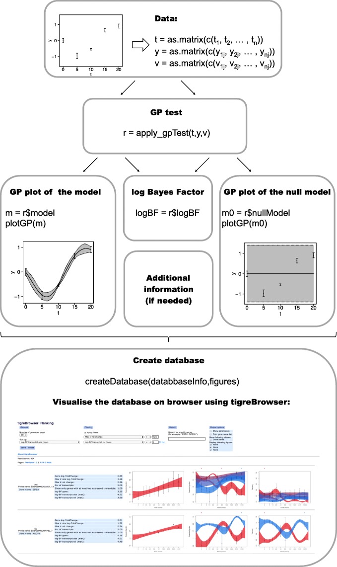
Fig. 3.
Schema displaying the use of GPrank functions. Time series data of each genetic element in the data set are represented by three one-column matrices: t: time points; y: estimated abundances at the corresponding time points; v: variances of the estimated abundances at the corresponding time points. These matrices are then given as input to the apply_gpTest() function. apply_gpTest() function optimises the time-dependent (m) and time-independent (m0) models and computes the natural logarithm of BF. The kernel structures are specified by default as (“rbf”, “white”, “fixedvariance”) in the time-dependent model, and as (“white”, “fixedvariance”) in the time-independent model. Fitted GP models can be plotted by plotGP() function. Finally, an SQL database can be created with createDatabase() function, allowing inclusion of the figures and additional information (e.g., BFs, fold changes) for visualisation, ranking, and filtering purposes. The created database can be viewed using tigreBrowser [30]

