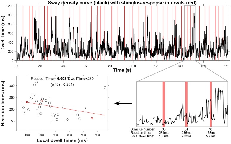
Figure 2.

Procedure outlining the posturographic analyses from global to local dwell-time estimation, and their relation to stimulus-response reaction times. The top panel displays the sway density curve, with in red the 41 episodes corresponding to stimulus-response intervals. Over the whole trial, the dwell time was on average 248 ms, but dwell times clearly fluctuate throughout the trial, with peaks up to 1,000 ms. In the lower-right panel, the sway-density curve is depicted for a period of about 10 s, containing three stimulus-response pairs (numbers 33, 34, and 35). As can be seen, the local dwell times taken over the stimulus-response intervals, as well as the reaction-time values, vary. This is confirmed by the negative correlation between local dwell times and reaction times, as depicted in the lower-left panel, with the linear fit (red line) and its regression equation yielding an overall negative slope (presented in bold font) for this trial.