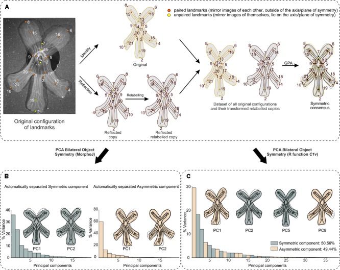
FIGURE 5.

Workflow for shape analysis of bilateral object symmetry in F. graciliflora (case study 1). (A) First, an original configuration is considered, then a reflected copy is generated and relabelled with the landmarks that are mirror images of each other with respect to the axis (or plane) of symmetry are mutually swapped (paired landmarks) while the ones that lie on the symmetry axis are mapped onto themselves (unpaired landmarks). A Generalised Procrustes Analysis is applied to this doubled dataset to extract shape data (Procrustes coordinates) by removing extraneous information of size, location and orientation via a least-squares criterion. The mean shape (consensus) is symmetric. (B) MorphoJ’s implementation of bilateral object symmetry automatically separates a component of symmetric variation (i.e., variation among flowers) from the asymmetry (i.e., variation within flowers or between left and right sides of flowers). Consequently, separate PCAs are run on the covariance matrix of the Procrustes coordinates for each component to quantify and display their patterns of shape changes, but do not indicate how much these PCs account for the total amount of shape variation. For each component, percentages of variance for which the PCs account are reported and the first 2 PCs and displayed. The outline drawings of flowers show shape changes associated with each PC from the overall average shape (dotted outline and open circles) for PC1 and PC2 scores of +0.1 (solid black outline with gray background and solid black circles). Note that these outline drawings are an interpolated form of display from the real landmarks based on the thin-plate spline method that makes it easier to visualise shape changes. This means that the interpretable information is from the positions of the landmarks, not from the outline drawings. (C) A PCA applied on the same superimposed already doubled dataset obtained via function ‘C1v’ unambiguously separates these components of shape variation and indicates how much their associated PCs account for the total variance. The first two PCs of each component are displayed. The outline drawings are generated as in (B).