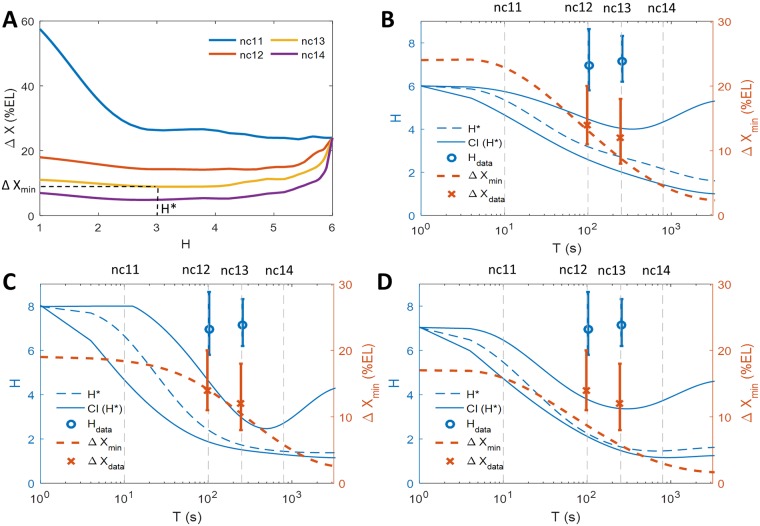
Fig 4. The positional resolution of the expression pattern for different nuclear cycles and regulatory models.
(A) Positional resolution calculated from the equilibrium binding site model with randomized kinetic parameters that give different values of the expression profile steepness H for M = 1. The colored lines show the results for parameters that give the smallest readout error CVP from a set of randomized parameters for the steady-state window T in nc 11-14 (Fig 2A). The curves are smoothed using cubic spline interpolation for better visualization. For each nuclear cycle we find the optimal Hill coefficient H* that results in a model with the smallest value of positional resolution, ΔXmin. (B-D) The range of optimal Hill coefficients H* (dashed blue line) that yield the lowest value of the positional resolution (obtained as described in Fig. 4A) as a function of the steady-state readout duration T for the equilibrium N = 6 model (defined in Eq 2 and S1D Text) (B); the hybrid N = 6 non-equilibrium model with 3 equilibrium and 3 non-equilibrium OS (defined in S1G Text) (C); and the two mirror TF gradient model (defined in S1H Text)(D). Around the optimal Hill coefficients H* that give the minimal value of the positional resolution ΔX (dashed blue line) we also plot the range of Hill coefficients that come from models resulting in ΔX = ΔXmin ± 2% EL, allowing for a tolerance interval for the positional resolution (solid blue lines). The curves are smoothed by cubic spline interpolation for better visualization. Also shown is the lowest achievable value of the positional resolution in the numerical randomization experiment for varying T (dashed orange line). The results are obtained assuming a diffusion limited estimate for τbind = 4s. The theoretical results for M = 1 for all models are compared to the empirical Hill coefficient Hdata (blue circles with error bars) and positional resolution ΔXdata (orange crosses with error bars) extracted from MS2-MCP live imaging data in nc 12 and nc 13 [13] (see S1I Text). The error bars correspond to 95% confidence intervals. In general, only the non-equilibrium model with N = 6 is able to produce both Hill coefficients and ΔX values observed in experiments. However, assuming tbind = 4s, even the non-equilibrium model cannot achieve the experimental values of the Hill coefficient during the time T of nc 12-13.

