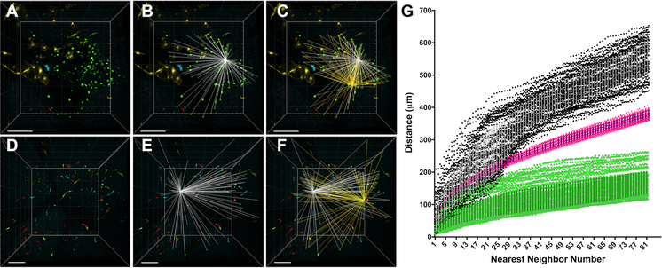
Figure 2. Nearest neighbor (NN) analysis as a quantitative comparison of the 3D distribution of confetti labeled ECs in CCMs, control brain slices, and computer simulations.

(A) 3D reconstruction of the entire volume of a CCM containing clonally dominant ECs labeled with nGFP. This CCM corresponds to CCM #23 in Figure 1K. (B) Visual representation of the 3D distances (white) between one EC and all of the other ECs within the CCM. The NN algorithm calculates and ranks these distances from closest to furthest. (C) Visual representation of the 3D distances (yellow) between a second EC and all of the other ECs within the CCM superimposed on the 3D distances of the first EC (white). (D-F) The same NN analysis is applied to non-CCM control brain slices: (D) 3D reconstruction of the control brain slices, (E) NN distances (white) between one nGFP EC and all of the other nGFP ECs, (F) a second set of NN distances (yellow) for a different nGFP EC and all of the nGFP ECs within the sample. (G) All of the NN distances, two of which are visually represented on the 3D reconstructions above, are ranked from closest to furthest and plotted as distance (μm) by NN number. The green data points represent the NN distances for all of the nGFP ECs within the CCM shown in panel A. The black data points represent the NN distances for all of the nGFP ECs within the control brain slices shown in panel D. The pink data points represent the average NN distances from 100 computer simulations in which the x,y,z coordinates of each member of the analysis were assigned by a random number generator. The simulation used the same volume and number of members (ECs) as the experimental CCM sample shown in panel A (error bars represent mean + SD). All scale bars are 100μm.