COMPUTER-AIDED DETECTION OF PATTERN CHANGES IN LONGITUDINAL ADAPTIVE OPTICS IMAGES OF THE RETINAL PIGMENT EPITHELIUM

Abstract

Retinal pigment epithelium (RPE) defects are indicated in many blinding diseases, but have been difficult to image. Recently, adaptive optics enhanced indocyanine green (AO-ICG) imaging has enabled direct visualization of the RPE mosaic in the living human eye. However, tracking the RPE across longitudinal images on the time scale of months presents with unique challenges, such as visit-to-visit distortion and changes in image quality. We introduce a coarse-to-fine search strategy that identifies paired patterns and measures their changes. First, longitudinal AO-ICG image displacements are estimated through graph matching of affine invariant maximal stable extremal regions in affine Gaussian scale-space. This initial step provides an automatic means to designate the search ranges for finding corresponding patterns. Next, AO-ICG images are decomposed into superpixels, simplified to a pictorial structure, and then matched across visits using tree-based belief propagation. Results from human subjects in comparison with a validation dataset revealed acceptable accuracy levels for the level of changes that are expected in clinical data. Application of the proposed framework to images from a diseased eye demonstrates the potential clinical utility of this method for longitudinal tracking of the heterogeneous RPE pattern.

1. INTRODUCTION

The retinal pigment epithelium (RPE) is an important tissue layer that nourishes and maintains retinal visual cells necessary for vision. RPE defects can result in loss of vision in disease [1]. Recently, we have shown that adaptive optics enhanced indocyanine green (AO-ICG) imaging can be used to visualize the RPE cell mosaic in living human eye [2]. The RPE mosaic has a heterogeneous appearance consisting of dark, gray, and bright patches (Fig. 1). Detection of changes to this underlying pattern can potentially reveal changes to the RPE indicating disease progression. This paper aims to develop a computer-aided detection framework to identify such changes.

Figure 1.

Image displacement computation in a longitudinal AO-ICG image pair by graph matching of affine invariant MSER correspondences. Green ellipses: MSERs; yellow +’s, MSER centroids; red lines: MSER feature correspondences. Local image distortion is illustrated by different ellipse shapes and angles corresponding to the same region (e.g. white arrow). Scale bar: 50μm.

Detection of pattern changes on longitudinal AO-ICG images is challenging for a number of reasons. First, variation in image quality or the locations of the imaged areas themselves can occur across a time window of several months. These are exacerbated by local distortions due to scanning or eye motion-induced artifacts, and also errors in the registration of overlapping images within the same imaging session. Finally, the RPE pattern is often degraded by noise. To overcome these challenges, we developed a coarse-to-fine search strategy to detect pattern changes. Image displacement is first estimated through graph matching of affine invariant maximal stable extremal regions (MSER) [3] in affine Gaussian scale-space. Next, patterns are represented as superpixels and then simplified to pictorial structures. Constrained by image displacement, local superpixel displacements are estimated through a tree-based belief propagation. Finally, these displacements guide superpixel pairing, which can be used to measure their pattern changes in longitudinal AO-ICG images.

2. METHODS

2.1 Image Displacement Estimation

The purpose of this step is to estimate image displacements between longitudinal AO-ICG images. These displacements are used to initialize the estimation of local pattern displacements described in the next section, and to automate the determination of search ranges.

AO-ICG images are first smoothed to reduce noise using total variation flow [4]. The MSER detector is then used to search for dark and bright regions in the smoothed images (green ellipses, Fig. 1). SIFT feature descriptor [5] is employed to describe each MSER, and image displacements are estimated by matching feature descriptors. However, it is inaccurate to directly establish feature descriptors on MSERs because image distortion often causes the same MSER to deform in the AO-ICG image pair, (e.g. Fig. 1, white arrows). To reduce image distortion errors, we adapt affine Gaussian scale-space [6,7] to estimate local affinity and compute feature descriptors on the affine invariant MSERs.

Let I(p), p = (x, y)^T, be an AO-ICG image,

$$L(\mathit{p};{\mathbf{\Phi }}_t)=g(\mathit{p};{\mathbf{\Phi }}_t)\ast I(\mathit{p}).$$ (1)

Here, Φ_t is a symmetric positive semi-definite matrix,

$$g(\mathit{p};{\mathbf{\Phi }}_t)=\frac{1}{2\pi \sqrt{\det {\mathbf{\Phi }}_t}}{e}^{-{\mathit{p}}^T{\mathbf{\Phi }}_t\mathit{p}/2}.$$ (2)

Assuming S(p₁) and S(p₂) are two corresponding MSERs with A as their affine transformation matrix, we can get p₂ = Ap₁. Supposing Φ_t,₁ and Φ_t,₂ are their affine Gaussian scale matrices, then according to affine Gaussian scale-space [6]:

$${\mathbf{\Phi }}_{t,1}={\mathbf{A}}^T{\mathbf{\Phi }}_{t,2}\mathbf{A}.$$ (3)

To estimate Φ_t, we apply the second moment matrix M to compute local affinity.

$$\mathbf{M}(\mathit{p};{\mathbf{\Phi }}_t)=g(\mathit{p};{\mathbf{\Phi }}_s)\ast (\nabla L(\mathit{p};{\mathbf{\Phi }}_t))\cdot (\nabla L{(\mathit{p};{\mathbf{\Phi }}_t)}^T).$$ (4)

Here, the integration scale matrix is defined as Φ_s = αΦ_t where α is a constant. Again, we can derive

$${\mathbf{M}}_2={\mathbf{A}}^{-T}{\mathbf{M}}_1{\mathbf{A}}^{-1}.$$ (5)

According to Eq. (3) and (5), we can get Φ_t = βM⁻¹, where β is a constant. The affine transform matrix A can be computed in terms of M,

$$\mathbf{A}={\mathbf{M}}_2^{-1/2}\mathbf{R}{\mathbf{M}}_1^{1/2}.$$ (6)

R is an orthogonal matrix which includes rotation and mirror transformations. Corresponding MSERs can be rewritten as

$${\mathit{p}}_2={\mathbf{M}}_1^{-1/2}\mathbf{R}{\mathbf{M}}_1^{1/2}{\mathit{p}}_1\Rightarrow {\mathbf{M}}_2^{1/2}{\mathit{p}}_2=\mathbf{R}{\mathbf{M}}_1^{1/2}{\mathit{p}}_1.$$ (7)

It is important that they should contain the same image contents under affine image distortion. We can adjust corresponding MSERs as ${\overline{\mathit{p}}}_1={\mathbf{M}}_1^{1/2}{\mathit{p}}_1$ and ${\overline{\mathit{p}}}_2={\mathbf{M}}_2^{1/2}{\mathit{p}}_2$ because corresponding adjusted MSERs only have orthogonal transforms which are affine invariant. This allows us to build accurate SIFT feature descriptors on the adjusted MSERs.

Graph matching [8] is used to find affine invariant MSER correspondences. Besides similarity values between SIFT feature descriptors, graph matching also combines geometric compatibility between MSER correspondences and uniqueness of correspondence into a unified framework. Together, these improve the matching in the presence of image distortions. Fig. 1 illustrates the final MSER corresponding results (red lines). Image displacements can be represented as ℒ_g = {l_g,₁, ⋯, l_g,_m}, where l_g,_i is the displacement vector between i-th corresponding MSERs.

2.2 Superpixel Displacement Computation

Image displacements provide an initial estimation of pattern correspondences in longitudinal AO-ICG images. Unfortunately, they often produce inaccurate correspondences due to local image distortions, which thereby necessitates a more refined computation of local pattern displacements. However, instead of computing all possible point correspondences, we introduce a tree-based belief propagation method that utilizes image displacements to initialize the search range of pattern correspondences, significantly reducing computational cost.

The heterogeneous pattern can be represented as a collection of smaller regions with homogeneous intensity. Homogeneous regions can be extracted using superpixels [9]. Estimation of local image displacements can thus be solved via determination of superpixel pairings between two images (e.g. Figs 2A and 2B). This problem can again be solved using graph matching [8]. However, graph matching used in estimating image displacement enforces unique correspondence, and the problem here involves many-to-one superpixel correspondence. Instead, we treat this problem as the minimization of pictorial structure through belief propagation [10], and use computed superpixel displacements to guide the subsequent pairing of superpixels.

Figure 2.

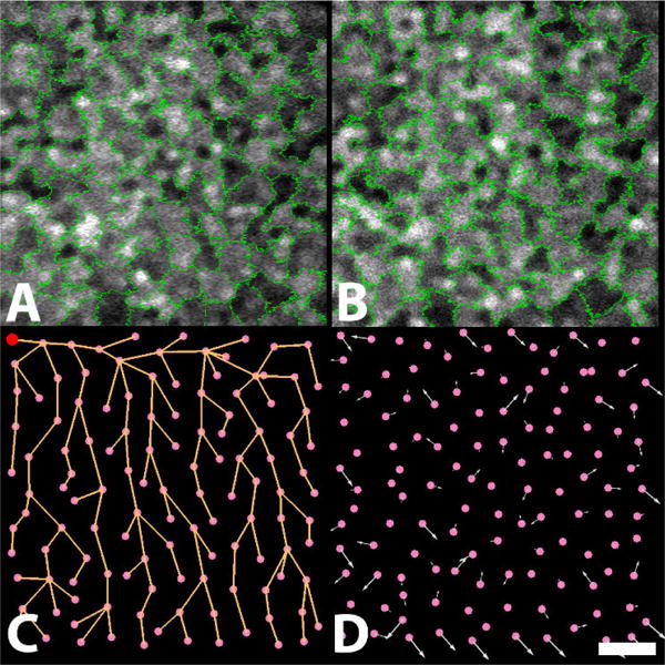
Superpixel displacement computation on a longitudinal image pair. Superpixel decompositions on the AO-ICG image from the (A) first and (B) second visits; (C) tree structure of superpixels from the first visit (red circle, tree root); (D) superpixel displacements of the first visit with respect to the second visit (arrows; lengths indicate amounts of displacement). Scale bar: 50μm.

Let G = (V, E) be the graph structure in Fig. 2A, and V = {v₁, ⋯, v_n} their node representations, where v_i corresponds to i-th superpixel. E includes all adjacent relationships between two superpixels in Fig. 2A. A configuration ℒ_s = {l_s,l, ⋯, l_s,_n} specifies a displacement vector for each superpixel v_i ∈ V. Superpixel displacement computation can be described as:

$${\overline{\mathrm{ℒ}}}_{\mathbf{s}}=\underset{{\mathrm{ℒ}}_s}{\arg min}\left({\displaystyle {\sum }_{v_i\in V}D({\mathit{l}}_{s,i},I)}+{\displaystyle {\sum }_{(v_i,v_j)\in E}F({\mathit{l}}_{s,i},{\mathit{l}}_{s,j})}\right),$$ (8)

where D (l_s,_i, I) measures how well the superpixel in Fig. 2A matches Fig. 2B when moved by l_s,_i. To reduce the computational cost, the census transform [11] is used as the similarity measurement for D(l_s,_i, I). F(l_s,_i, l_s,_j) = |l_s,_i − l_s,_j|² measures how continuous two displacement vectors from adjacent superpixels are with each other.

However, minimizing an arbitrary graph of Eq. (8) is an NP-hard problem. Additionally, the continuity assumption is often not fulfilled between adjacent superpixels. We reduce the graph structure in Eq. (8) into a minimum-spanning tree [12] (Fig. 2C). The root is arbitrarily selected (red circle, Fig. 2C). Weights of the graph structure are census transform values because we assume that adjacent superpixels with similar visual appearance are more likely to have similar displacement vectors in Fig. 2A.

Dynamic programming is used to efficiently minimize Eq. (8) on the tree structure. Starting with a leaf node v_j, the matching value of the best displacement vector of l_s,_j given the displacement vector l_s,_i of its parent node v_i is

$$Y_j({\mathit{l}}_{s,i})=\underset{{\mathit{l}}_{s,j}}{min}\left(D({\mathit{l}}_{s,j},I)+F({\mathit{l}}_{s,i},{\mathit{l}}_{s,j})\right).$$ (9)

Here, l_s,_i is initialized by an image displacement vector l_g ∈ ℒ_g in the previous section where the MSER is close to the current superpixel. Meanwhile, the search range of l_s,_j is also limited by max(ℒ_g). Therefore, we can apply image displacements to initialize the computation and automate the determination of search ranges. Iteratively, we can compute the remaining tree nodes, other than the root.

$$Y_j({\mathit{l}}_{s,i})=\underset{{\mathit{l}}_{s,r}}{min}(D({\mathit{l}}_{s,j},I)+F({\mathit{l}}_{s,i},{\mathit{l}}_{s,j})+{\sum }_{v_c\in C_j}{Y}_c({\mathit{l}}_{s,j})).$$ (10)

Here, the last term is known as we always compute child nodes first. Eventually, we reach the root. If all its child nodes are known, we can compute its displacement vector as

$${\overline{\mathit{l}}}_{s,r}=\underset{{\mathit{l}}_{s,r}}{\arg min}\left(D({\mathit{l}}_{s,j},I)+{\displaystyle {\sum }_{v_c\in C_j}{Y}_c({\mathit{l}}_{s,j})}\right).$$ (11)

Starting from the root, we can work reversely to determine the displacement vectors of all tree nodes until all leaf nodes are reached by changing the computation from ‘min’ in Eq. (9) and (10) to ‘argmin’. Superpixel displacements are illustrated as white arrows in Fig. 2D.

2.3 Determination of Pattern Changes

Each superpixel in the first visit (Fig. 2A) is translated to the second visit through its displacement vector. This can cover a set of superpixels in the second visit. We choose the one with the largest number of overlapping pixels as its counterpart. The mean intensities m₁ and m₂ are computed for the paired superpixels. If m₂ > m₁ + γ, pattern changes are marked as having changed from dark to bright; m₂ < m₁ − γ, bright to dark; otherwise, stable. Here, γ is the sensitivity threshold. Since we are interested in detecting only significant changes (e.g. from bright to dark as opposed to from dark to darker, and vice versa), we empirically set γ = 80 in this paper.

2.4 Dataset Collection

Research procedures adhered to the tenets of the Declaration of Helsinki and were approved by the Institutional Review Board of the National Institutes of Health. Since AO-ICG was first introduced in 2016 [2], there is limited AO-ICG data available. To the best of our knowledge, we present for the first time longitudinal AO-ICG data in four subjects (3 healthy, 1 patient with late-onset retinal degeneration). The time between imaging sessions was 3–4 months for the healthy subjects and 12 months for the patient. A total of 669 overlapping small field-of-view videos were recorded in these subjects, corrected for eye motion artifacts, and combined to create larger RPE images. We created validation datasets from the healthy subjects to evaluate the robustness and accuracy of the detection framework. For each subject, we selected two RPE regions (6 regions total). First, for each RPE region, we generated an image pair, each with a unique distortion due to eye motion (400×400 pixels). Second, for each RPE region, we artificially introduced two types of modifications to the pattern: (1) changing intensity values by 150 (0–255 intensity range; bright regions were made darker, and dark regions brighter), and (2) inverting the intensities (255− I). For the test dataset, we collected image pairs (1000×1000 pixels) in two RPE regions for each of the four subjects.

3. EXPERIMENTAL RESULTS

3.1 Validation Datasets

Detection accuracy was defined as the ratio between total areas of superpixels in the first image that successfully paired counterparts in the second image (whether or not a change was truly made), divided by the total area of the unchanged image plane. No changes were detected across all six image pairs in the case of the first validation dataset, in which the only differences between images were different sets of image distortion due to eye motion and scanning. This establishes that our approach is robust to local distortion. For the second validation dataset, detection accuracies with increasing levels of changes are summarized in Table 1 (mean±standard deviation). The detection accuracy is higher in the case of changing intensities vs. inverting the values. This is potentially due to the census transform being more robust to a constant intensity change than to the inverse change. The overall drop in accuracy with increasing area change ratio is likely due to the creation of substantially different trees due to splitting or merging of superpixel areas resulting from the two operations (change and invert). These results indicate high accuracy for area change ratios within 15%. This drop-off in accuracy at larger change ratios is a tradeoff that is needed for the gain in computational speeds realized by the simplification of the superpixels to the tree structure.

Table 1.

Detection accuracy of relative area ratio versus area change ratio of manual intensity operations.

Operation	Area change ratio
	5%	10%	15%	20%	25%
Change (%)	98.6 ±0.9	97.2 ±1.2	94.9 ±1.9	91.5 ±3.1	85.7 ±2.7
Invert (%)	98.4 ±0.4	96.1 ±0.6	92.2 ±1.1	88.3 ±3.1	83.9 ±3.4

3.2 Test Dataset

For the test dataset, the average computation time was 14.4±2.6 seconds for 1000×1000 pixel AO-ICG images. As expected, detection results on six images pairs from three healthy subjects showed minimal changes across visits (area change ratio of 0.2±0.3%, mean±standard deviation). Detected changes were typically found near the boundaries of images (Fig 3A–C). There were no regions observed with intensity increase in three healthy subjects, while intensity decrease was observed in two image pairs. In contrast, several changes in the RPE pattern were found in the diseased eye with both intensity increases and decreases (Figs. 3D–3F). The overall area change ratio for this patient was 5.2%. Based on our validation results, we estimate that our algorithm can detect with high accuracy changes to the RPE mosaic when the visit-to-visit area change ratio is within 15%. Therefore, these changes are likely to be indicative of disease progression.

Figure 3.

Detection results of pattern changes on a healthy subject (top row) and a patient with late-onset retinal degeneration (bottom row). Left column: AO-ICG images from the first visit; center column: the second visit after 3 months (top row) and 12 months (bottom row); right column: pattern change maps overlaid with superpixel displacements, where intensity increase (red), decrease (blue), and stable (green). Superpixel displacements indicate the local region movements between AO-ICG images from the first visit to the second. Three regions of pattern changes are highlighted by circles. Scale bar: 50μm.

4. CONCLUSION AND FUTURE WORK

In this paper, we developed a computer-aided detection framework to identify pattern changes in a novel dataset of longitudinal AO-ICG images. This framework was based on a coarse-to-fine strategy to estimate image displacement and uses a simple, computationally-efficient method to determine correspondences between superpixel regions across different visits. Our proposed algorithm is robust against local distortions that arise from the combination of scanning and eye motion and is accurate for total area changes across visits of up to 15%. As expected, evaluation in a test dataset of healthy subjects revealed little to no change. Application to two image pairs from a patient revealed a 5.2% change to the RPE mosaic across a one-year time window, suggestive of the rate of disease progression.

The proposed framework sometimes yielded false matches when there was significant local image displacement due to errors in registration between overlapping images or degradation of image quality in portions of the image, particularly for the patient data. Such detection errors could be potentially due to the insufficient discriminative capability of the census transform. Further testing on additional patient datasets will help to further improve the robustness of this algorithm. In the future, development of a more discriminative feature descriptor that is computationally inexpensive will lead to improvements in performance. In addition, evaluation of this framework in a larger AO-ICG database with more healthy subjects and patients will also be important. All in all, longitudinal evaluation of changes to the RPE together with tracking of other retinal neurons [8] may lead to new insights about the onset and progression of blinding retinal diseases.

References

- 1.Sparrow JR, Hicks D, Hamel CP. The Retinal Pigment Epithelium in Health and Disease. Current Molecular Medicine. 2005 Jul;10(9):802–823. doi: 10.2174/156652410793937813. [DOI] [PMC free article] [PubMed] [Google Scholar]
- 2.Tam J, Liu J, Dubra A, Fariss R. In Vivo Imaging of the Human Retinal Pigment Epithelial Mosaic Using Adaptive Optics Enhanced Indocyanine Green Ophthalmoscopy. Investigative Ophthalmology & Visual Science. 2016 Aug;57(10):4376–4384. doi: 10.1167/iovs.16-19503. [DOI] [PMC free article] [PubMed] [Google Scholar]
- 3.Nister D, Stewenius H. Linear Time Maximally Stable Extremal Regions. Proc 10th European Conference on Computer Vision. 2008 Oct;5303:183–196. [Google Scholar]
- 4.Steidl G, Weickert J, Brox T, Mrazek P, Welk M. On the Equivalence of Soft Wavelet Shrinkage, Total Variation Diffusion, Total Variation Regularization, and SIDEs. SIAM Journal on Numerical Analysis. 2004 May;42(2):686–713. [Google Scholar]
- 5.Lowe DG. Distinctive Image Features from Scale-invariant Keypoints. International Journal of Computer Vision. 2004 Nov;60(2):91–110. [Google Scholar]
- 6.Lindeberg T. Generalized Gaussian Scale-space Axiomatics Comprising Linear Scale-space, Affine Scale-space and Spatiotemporal Scale-space. Journal of Mathematical Imaging and Vision. 2011 May;40(1):36–81. [Google Scholar]
- 7.Mikolajczyk K, Schmid C. Scale & Affine Invariant Interest Point Detectors. International Journal of Computer Vision. 2004 Oct;60(1):63–86. [Google Scholar]
- 8.Liu J, Jung H, Tam J. Accurate Correspondence of Cone Photoreceptor Neurons in the Human Eye Using Graph Matching Applied to Longitudinal Adaptive Optics Images. International Conference on Medical Image Computing and Computer-Assisted Intervention. 2017 Sep;10434:153–161. doi: 10.1007/978-3-319-66185-8_18. [DOI] [PMC free article] [PubMed] [Google Scholar]
- 9.Achanta R, Shaji A, Smith K, Lucchi A, Fua P, Susstrunk S. SLIC Superpixels Compared to State-of-art Superpixel Methods. IEEE Transactions on Pattern Analysis and Machine Intelligence. 2012 May;34(11):2274–2282. doi: 10.1109/TPAMI.2012.120. [DOI] [PubMed] [Google Scholar]
- 10.Felzenszwalb P, Huttenlocher D. Pictorial Structures for Object Recognition. International Journal of Computer Vision. 2005 Jan;61(1):55–79. [Google Scholar]
- 11.Zabih R, Woodfill J. Non-parametric Local Transforms for Computing Visual Correspondence. Proc 3rd European Conference on Computer Vision. 1994 May;801:151–158. [Google Scholar]
- 12.Prim RC. Shortest Connection Networks And Some Generalizations. Bell System Technical Journal. 1957 Nov;36(6):1389–1401. [Google Scholar]