Neural representation of vowel formants in tonotopic auditory cortex

Abstract

Speech sounds are encoded by distributed patterns of activity in bilateral superior temporal cortex. However, it is unclear whether speech sounds are topographically represented in cortex, or which acoustic or phonetic dimensions might be spatially mapped. Here, using functional MRI, we investigated the potential spatial representation of vowels, which are largely distinguished from one another by the frequencies of their first and second formants, i.e. peaks in their frequency spectra. This allowed us to generate clear hypotheses about the representation of specific vowels in tonotopic regions of auditory cortex. We scanned participants as they listened to multiple natural tokens of the vowels [ɑ] and [i], which we selected because their first and second formants overlap minimally. Formant-based regions of interest were defined for each vowel based on spectral analysis of the vowel stimuli and independently acquired tonotopic maps for each participant. We found that perception of [ɑ] and [i] yielded differential activation of tonotopic regions corresponding to formants of [ɑ] and [i], such that each vowel was associated with increased signal in tonotopic regions corresponding to its own formants. This pattern was observed in Heschl’s gyrus and the superior temporal gyrus, in both hemispheres, and for both the first and second formants. Using linear discriminant analysis of mean signal change in formant-based regions of interest, the identity of untrained vowels was predicted with ~73% accuracy. Our findings show that cortical encoding of vowels is scaffolded on tonotopy, a fundamental organizing principle of auditory cortex that is not language-specific.

1. Introduction

Cortical encoding of speech sounds has been shown to depend on distributed representations in auditory regions on Heschl’s gyrus (HG) and the superior temporal gyrus (STG). Studies using functional MRI (Formisano et al., 2008; Obleser et al., 2010; Kilian-Hutten et al., 2011; Bonte et al., 2014; Arsenault and Buchsbaum, 2015; Evans and Davis, 2015; Zhang et al., 2016) and intracranial electrocorticography (Chang et al., 2010; Pasley et al., 2012; Chan et al., 2014; Mesgarani et al., 2014; Leonard et al., 2016; Moses et al., 2016) have shown that phonemes can be reconstructed and discriminated by machine learning algorithms based on the activity of multiple voxels or electrodes in these regions. Neural data can distinguish between vowels (Formisano et al., 2008; Obleser et al., 2010; Bonte et al., 2014; Mesgarani et al., 2014) and between consonants (Chang et al., 2010; Mesgarani et al., 2014; Arsenault and Buchsbaum, 2015; Evans and Davis, 2015), and there is evidence that phonemic representations in these regions are categorical and reflect the contribution of top-down information (Chang et al., 2010; Kilian-Hutten et al., 2011; Bidelman et al., 2013; Mesgarani et al., 2014; Leonard et al., 2016).

However, little is known regarding the spatial organization of cortical responses that underlie this distributed encoding, even in cases where hypotheses can readily be made based on known principles of auditory cortical organization. The most prominent organizing principle of core auditory regions is tonotopy, whereby there are several continuous gradients between regions in which neurons preferentially respond to lower or higher frequencies (Talavage and Edmister, 2004; Woods et al., 2009; Humphries et al., 2010; Da Costa et al., 2011; Dick et al., 2012; Saenz and Langers, 2014; De Martino et al., 2015). Tonotopic organization also extends to auditory regions beyond the core on the lateral surface of the STG and beyond (Striem-Amit et al., 2011; Moerel et al., 2012, 2013; Dick et al., 2017).

Vowels are pulse-resonance sounds in which the vocal tract acts as a filter, imposing resonances on the glottal pulses, which appear as peaks on the frequency spectrum. These peaks are referred to as formants, and vowels are distinguished from one another largely in terms of the locations of their first and second formants (Peterson and Barney, 1952), which are quite consistent across speakers despite variation in the pitches of their voices, and across pitches within each individual speaker. Because formants are defined in terms of peak frequencies, we hypothesized that vowels may be discriminable based on neural activity in tonotopic regions corresponding to the formants that characterize them.

In animal studies, perception of vowels is associated with increased firing rates of frequency-selective neurons in primary auditory cortex (Versnel and Shamma, 1998; Mesgarani et al., 2008). In humans, natural sounds are encoded by multiple spectrotemporal representations that differ in spatial and temporal resolution (Moerel et al., 2012, 2013; Santoro et al., 2014) such that spectral and temporal modulations relevant for speech processing can be reconstructed from functional MRI data acquired during presentation of natural sounds (Santoro et al., 2017). Therefore it can be predicted that the cortical encoding of vowels, as a special case of natural sounds, would follow the same principles. However, the cortical representation of vowel formants in tonotopic regions has not previously been demonstrated. Magnetoencephalography (MEG) studies have shown differences in source localization between distinct vowels (Obleser et al., 2003, 2004; Scharinger et al., 2011), but findings have been inconsistent across studies (Manca and Grimaldi, 2016), so it is unclear whether any observed differences reflect tonotopic encoding of formants. Neuroimaging studies have almost never reported activation differences between different vowels in univariate subtraction-based analyses (e.g. Formisano et al., 2008; Obleser et al., 2010). As noted above, the imaging and electrocorticography studies that have demonstrated neural discrimination between vowels have done so on the basis of distributed representations (e.g. Formisano et al., 2008; Mesgarani et al., 2014). The patterns of voxels or electrodes contributing to these classifications have been reported to be spatially dispersed (Mesgarani et al., 2014; Zhang et al., 2016).

To determine whether vowel formants are encoded by tonotopic auditory regions, we used functional MRI to map tonotopic auditory cortex in twelve healthy participants, then presented blocks of the vowels [ɑ] (the first vowel in ‘father’) and [i] (as in ‘peak’) in the context of an irrelevant speaker identity change detection task. We examined neural responses to the two vowels in regions of interest where voxels’ best frequencies corresponded to their specific formants, to determine whether vowel identity could be reconstructed from formant-related activation.

2. Materials and methods

2.1. Participants

Twelve neurologically normal participants were recruited from the University of Arizona community in Tucson, Arizona (age 32.0 ± 5.9 (sd) years, range 26–44 years; 7 male, 5 female; all right-handed; all native speakers of English; education 17.8 ± 1.6 years, range 16–20 years). All participants passed a standard hearing screening (American Speech-Language-Hearing Association, 1997).

All participants gave written informed consent and were compensated for their time. The study was approved by the institutional review board at the University of Arizona.

2.2. Structural imaging

MRI data were acquired on a Siemens Skyra 3 Tesla scanner with a 32-channel head coil at the University of Arizona. A whole-brain T1-weighted magnetization-prepared rapid acquisition gradient echo (MPRAGE) image was acquired with the following parameters: 160 sagittal slices; slice thickness = 0.9 mm; field of view = 240 × 240 mm; matrix = 256 × 256; repetition time (TR) = 2.3 s; echo time (TE) = 2.98 ms; flip angle = 9°; GRAPPA acceleration factor = 2; voxel size = 0.94 × 0.94 × 0.94 mm.

Cortical surfaces were reconstructed from the T1-weighted MPRAGE images using Freesurfer version 5.3 (Dale et al., 1999) running on Linux (xubuntu 16.04). Four surface-based anatomical regions of interest (ROIs) were defined using automated cortical parcellation (Fischl et al., 2004). Specifically, HG and the STG were identified in the left and right hemispheres based on the Desikan-Killiany atlas (Desikan et al., 2006).

2.3. Tonotopic mapping

Two functional runs were acquired to map tonotopic regions of auditory cortex in each participant. To engage both primary and non-primary auditory areas in meaningful processing (Moerel et al., 2012), the stimuli consisted of bandpass-swept human vocalizations, as previously described by Dick et al. (2012). In brief, vocalization tokens were produced by actors who were instructed to express eight different emotions using the French vowel [ɑ] (Belin et al, 2008). The tokens were spliced together to form sequences of 8 m 32 s. These sequences were then bandpass filtered in eight ascending or descending sweeps of 64 s each. Each sweep involved a logarithmic ascent of the center frequency from 150 Hz to 9600 Hz, or a similar descent. Although the vocalization tokens used the vowel [ɑ], the filtering ensured that there was no trace of the formants of [ɑ] in the tonotopic stimuli. The stimuli were then filtered again to compensate for the acoustic transfer function of the earphones (see below), and were presented at a comfortable level for each participant. To ensure attention to the stimuli, participants were asked to press a button whenever they heard the sound of laughter, which was one of the eight emotional sounds. Additional details are provided in Dick et al. (2012).

Auditory stimuli were presented using insert earphones (S14, Sensimetrics, Malden, MA) padded with foam to attenuate scanner noise and reduce head movement. Visual stimuli (consisting only of a fixation crosshair for the tonotopic runs) were presented on a 24″ MRI-compatible LCD monitor (BOLDscreen, Cambridge Research Systems, Rochester, UK) positioned at the end of the bore, which participants viewed through a mirror mounted to the head coil. Button presses were collected via a fiber optic button box (Current Designs, Philadelphia, PA) placed in the right hand. Stimuli were presented and responses recorded with custom scripts written using the Psychophysics Toolbox version 3.0.10 (Brainard 1997; Pelli 1997) in MATLAB R2012b (Mathworks, Natick, MA).

One ascending run and one descending run were acquired. T2*-weighted BOLD echo planar images were collected with the following parameters: 256 volumes; 28 axial slices in interleaved order, aligned with the Sylvian fissure and spanning the temporal lobe; slice thickness = 2 mm with no gap; field of view = 220 × 220 mm; matrix = 110 × 110; repetition time (TR) = 2000 ms; echo time (TE) = 30 ms; flip angle = 90°; voxel size = 2 × 2 × 2 mm. An additional 10 volumes were acquired and discarded at the beginning of each run, to allow for magnetization to reach steady state and to avoid auditory responses to the onset of scanner noise.

The functional data were preprocessed with tools from AFNI (Cox, 1996). The data were resampled to account for differences in slice acquisition times. Head motion was corrected, with six translation and rotation parameters saved for use as covariates. In the course of head motion correction, all functional runs were aligned with the last volume of the last tonotopy run, which was acquired closest to the structural scan. Then the data were detrended with a Legendre polynomial of degree 2. The functional images were aligned with the structural images using bbregister in Freesurfer, and manually checked for accuracy. No spatial smoothing was applied to the functional data, except for rendering onto the cortical surface for visualization.

Tonotopic mapping data were analyzed with Fourier methods using Csurf (Sereno et al., 1995), whereby voxels preferentially responding to a particular point in the stimulus cycle will show a higher amplitude at the frequency of stimulus cycling (i.e. 1/64 Hz) than at any other frequency. The phase of the signal, which corresponds to a particular point of the stimulus ramp, is then mapped to the color wheel, while the amplitude of the signal is mapped to the voxel’s color saturation. Runs with downward frequency sweeps were time reversed and averaged with upward-swept scans to compensate for delays in the BOLD response (estimated to be a 0.08 fraction of the 64-second cycle, i.e. ~5 s).

2.4. Vowels task

Three functional runs were acquired to estimate cortical responses to the vowels [ɑ] and [i]. In each run, tokens of the vowels [ɑ] and [i] were presented repeatedly in a block design, to maximize signal to noise. All blocks were 16 s in duration, and each run comprised 10 [ɑ] blocks, 10 [i] blocks, and 10 silent blocks, as well as 16 s of silence at the beginning of the scan, and 12 s of silence at the end of the scan, for a total run duration of 8 m 28 s. Blocks were presented in pseudorandom order such that adjacent blocks never belonged to the same condition. Each vowel block contained 13 vowels, with an inter-stimulus interval of 1230 ms.

An oddball speaker detection task was used to ensure participants’ attention. Of the 260 vowels in each run, 240 were produced by a primary male speaker, and 20 (8.3%) by a different male speaker. The oddball stimuli were distributed equally across the [ɑ] and [i] conditions such that 30% of blocks contained no oddball stimuli, 40% contained one, and 30% contained two. Oddballs were never the first stimulus in the block, and if there were two oddballs in a block, they were not consecutive.

Participants were instructed to fixate on a centrally presented crosshair and press a button whenever they heard a vowel produced by the oddball speaker. Feedback was provided in the form of a small centrally presented green smiling face for hits (between 300 ms and 1530 ms post-onset) or a red frowning face for false alarms. To encourage close attention to the stimuli, participant payment amount was dependent on performance. The task was practiced prior to entering the scanner.

The vowels [ɑ] and [i] were selected because their first and second formants are maximally dissimilar (Peterson and Barney, 1952). Male speakers were used because their lower fundamental frequencies entail that harmonics are closer together, reducing the likelihood that formant peaks could fall between harmonics. The primary speaker and the oddball speaker were recorded in a soundproof booth with a Marantz PMD661 Portable Flash Field Recorder and a Sanken COS-11D Miniature Omnidirectional Lavalier Microphone. Each speaker was instructed to produce isolated natural tokens of [ɑ] and [i]. After several tokens of each vowel were produced, the best token of each vowel was selected to be used as a model. The models were played back to the speaker multiple times to be mimicked. In this way, multiple natural stimuli were obtained that were similar yet not identical. Thirty tokens of each vowel were selected from the primary speaker, and five of each from the oddball speaker.

The [i] vowels proved to be longer than the [ɑ] vowels, so [i] tokens were shortened by removing glottal pulses from the central portions of the vowels. After editing, the primary speaker’s [ɑ] durations were 737 ± 41 ms and his [i] durations were 737 ± 45 ms. The oddball speaker’s [ɑ] durations were 675 ± 22 ms and his [i] durations were 675 ± 22 ms. The stimuli were then filtered to compensate for the acoustic transfer function of the Sensimetrics earphones. Finally, all stimuli were normalized for root mean squared amplitude. Examples of [ɑ] and [i] tokens are shown in Figure 1A.

Figure 1.

Vowels used in the experiment. (A) Spectrograms and spectra of representative [ɑ] and [i] tokens. (B) Comparison between the [ɑ] and [i] spectra, showing how formant bands were defined.

The multiple tokens of each vowel were presented pseudorandomly. Each primary speaker vowel token was presented four times per run, and each oddball speaker vowel token was presented twice per run. In the scanner, stimuli were presented at a comfortable level for each participant.

The three vowel runs were acquired and preprocessed exactly as described for the tonotopy runs, except that there were 246 volumes per run. The vowel runs were modeled with two simple boxcar functions for the [ɑ] and [i] blocks, which were convolved with a canonical hemodynamic response function and fit to the data with a general linear model using the program fmrilm from the FMRISTAT package (Worsley et al., 2002). The six translation and rotation parameters derived from motion correction were included as covariates, as were three cubic spline temporal trends. The [ɑ] and [i] blocks were each contrasted to rest, and each participant’s three runs were combined in fixed effects analyses using multistat.

2.5. Responses to vowels in tonotopic regions

The pitch and formants of the vowels were measured using Praat (Boersma, 2001) based on median values for the middle third of each vowel. For the primary speaker, these measurements were as follows: f₀ = 98 ± 1 Hz; [ɑ] F₁ = 768 ± 7 Hz; [ɑ] F₂ = 1137 ± 41 Hz; [i] F₁ = 297 ± 16 Hz; [i] F₂ = 2553 ± 33 Hz. For the oddball speaker, the measurements were: f₀ = 115 ± 1 Hz; [ɑ] F₁ = 756 ± 9 Hz; [ɑ] F₂ = 1238 ± 153 Hz; [i] F₁ = 327 ± 6 Hz; [i] F₂ = 2123 ± 27 Hz.

Four “formant bands” were defined based on the formant peaks of the vowel stimuli (Figure 1B). In order to maximize signal to noise by including as many voxels as possible in formant-based ROIs, each band was defined to be as wide as possible without overlapping any adjacent bands. In cases where there was no relevant adjacent band, bands were defined to be symmetrical around their formant peaks. These calculations are described in detail in the following paragraphs.

The [i] F₁ peak was 297 Hz. The adjacent peaks of relevance were f₀ (peak = 98 Hz) and [ɑ] F₁ (peak = 768 Hz). Therefore the lower bound of the [i] F₁ band was defined as the logarithmic mean of 98 Hz and 297 Hz, which is 171 Hz, and the upper bound was defined as the logarithmic mean of 297 Hz and 768 Hz, which is 478 Hz. Logarithmic means were used to account for the non-linearity of frequency representation in the auditory system.

The [ɑ] F₁ peak was 768 Hz. The adjacent formants were [i] F₁ below and [ɑ] F₂ (peak = 1137 Hz) above. The lower bound of the [ɑ] F₁ band was defined as 478 Hz (the boundary with [i] F₁ as just described), and the upper bound was defined as the logarithmic mean of 768 Hz and 1137 Hz, which is 934 Hz.

The [ɑ] F₂ peak was 1137 Hz. The [ɑ] F₁ formant was adjacent below, so the lower bound of the [ɑ] F₂ band was defined as 934 Hz (as just described). There was no relevant formant immediately adjacent above, so the upper bound was set such that the [ɑ] F₂ band would be symmetrical (on a logarithmic scale) around the peak, i.e. the upper bound was defined as 1383 Hz.

The [i] F₂ peak was 2553 Hz. While no other first or second formants were adjacent above, the [ɑ] F₃ formant (peak = 2719 Hz) was adjacent above, so the upper bound of the [i] F₂ band was defined as the logarithmic mean of 2553 Hz and 2719 Hz, which is 2635 Hz. There was no relevant formant immediately adjacent below, so the lower bound for the [i] F₂ band was set such that the band would be symmetrical (on a logarithmic scale) around its peak, i.e., the lower bound was set to 2474 Hz.

Note that while all four formant bands showed differential energy for the two vowels, the difference in energy was considerably greater for the two [ɑ] formant bands (Figure 1B). This was due in part to energy from [ɑ] f₀ and F₃ impinging on the [i] F₁ and F₂ bands respectively.

The four formant bands ([ɑ] F₁, [i] F₁, [ɑ] F₂, [i] F₂) were crossed with the four anatomical ROIs (Left HG, Right HG, Left STG, Right STG, based on the Desikan-Killiany atlas) to create sixteen ROIs for analysis. Each ROI was constructed by identifying all voxels within each anatomical region that were tonotopic as reflected in a statistic of F > 3.03 (p < 0.05, uncorrected) in the phase encoded Fourier analysis, and had a best frequency within one of the four formant bands. ROIs were required to include at least two voxels. Because tonotopic regions can be small and somewhat variable across individuals, not all participants had at least two voxels in each ROI. In these instances, data points for the ROI(s) in question were coded as missing, although data points for the participants’ other ROIs were included.

To investigate responses to the two vowels in the four formant bands crossed by the four ROIs, a mixed model was fit using lme4 (Bates et al., 2015) in R (R Core Team, 2018). There were five fixed effects, each with two levels. Two effects pertained to the anatomical region of interest: region (HG, STG) and hemisphere (left, right). Two effects pertained to the formant band: the formant number (i.e. was the formant band defined based on the first or second formant?) and “ROI-defining vowel” (i.e. was the formant band defined based on spectral peaks of [ɑ] or [i]?). The fifth effect will be referred to as “presented vowel”, i.e. to which vowel was the response estimated? All main effects and full factorial interactions were included in the model. Participant identity was modeled as a random effect, with unique intercepts fit for each participant. The dependent measure was estimated signal change ($\widehat{\beta }$) relative to rest, averaged across the three runs and all voxels in the ROI. The primary effect of interest was the interaction of ROI-defining vowel by presented vowel, which tests the main study hypothesis. Also of interest were all higher level interactions involving ROI-defining vowel and presented vowel, in order to determine whether any patterns observed were modulated by region, hemisphere, or formant number. P values were obtained by likelihood ratio tests comparing models with and without each effect in question, including all higher level interactions that did not involve the effect in question. Null distributions for the likelihood ratio test statistic 2(l_F – l_R), where l_F is the log likelihood of the full model and l_R is the log likelihood of the reduced model, were derived using a parametric bootstrap approach (Faraway, 2016). Our study was adequately powered to detect large effects: with 12 participants, power was ≥ 80% for contrasts with an effect size of d ≥ 0.89 (two-tailed).

2.6. Classification of vowels based on neural data

The vowels task data were reanalyzed with one explanatory variable per vowel block, that is, 20 explanatory variables per run. In all other respects, the analysis was identical to that described above. Across the three runs, 60 estimates of signal changes in response to each block were obtained: 30 for [ɑ] blocks and 30 for [i] blocks.

Linear discriminant analysis (LDA) was used to determine whether the identity of blocks could be reconstructed from responses in the four formant bands in the four anatomical ROIs. From the fitted response to each block, a vector was derived encoding the mean response (across voxels) in each formant band in each ROI. These vectors had 16 elements, except for participants in whom one or more formant bands were not represented in all anatomical ROIs, as noted above. For each participant, each of the 60 blocks were left out in turn, and a discriminant analysis model was derived from the remaining 59 blocks using the fitcdiscr function in MATLAB 2017b. This model was then used to predict the identity of the held out block using the predict function.

Accuracy was calculated for each participant, and compared to chance (50%) across participants using a t-test. The question of whether classifier performance depended on ROIs being based on the formants of the vowels to be discriminated was addressed with respect to two different null permutations. In the first, four non-formant bands were defined that were the same logarithmic frequency width as the real formants, but were deliberately placed in parts of frequency space that should be less informative with respect to discriminating the two vowels. Specifically, the four non-formants were defined as: (1) 150–160 Hz (same width as [i] F₂): a region between f₀ and [i] F₁; (2) 341–668 Hz (same width as [ɑ] F₁): a region spanning [i] F₁ and [ɑ] F₁; (3) 1520–2251 Hz (same width as [ɑ] F₂): a region above [ɑ] F₂ and below [i] F₂ where neither vowel has much power; (4) 3412–9600 Hz (same width as [i] F₁): a region above F₃ of both vowels. In the second null permutation, the 150–9600 Hz frequency range was divided into 100 segments of equal width in logarithmic space, then 1000 permutations were run in which segments were randomly assigned to four non-formants which were again constrained to have the same logarithmic width (subject to rounding) as the real formants (i.e. the permuted [ɑ] F₁ was composed of 16 segments randomly chosen from the 100; [i] F₁: 25 segments, [ɑ] F₂: 9 segments; [i] F₂: 2 segments). Unlike the first null dataset, non-formants were not required to be contiguous in frequency space in this analysis, because permutations required to maintain contiguity would inevitably span informative regions where spectral power differs in many cases.

In order to determine whether some brain regions or formants were more informative than others for classification, several classifiers were constructed from subsets of the data. The following pairs of classifiers were compared: HG versus STG; left hemisphere versus right hemisphere; F₁ versus F₂ formants.

3. Results

3.1. Behavioral data

In the tonotopy task, participants detected 69.2 ± 19.4% of the instances of laughter (range 27.5–92.5%) embedded in the stimuli, while making a median of 25.5 false alarms (range 1–71) in total across the two runs. In the vowel task, participants detected 98.8 ± 1.4% of the oddball vowels (range 95–100%), while making a median of 2 false alarms (range 0–7) in total across the three runs. These results indicate that all participants maintained attention to the stimuli throughout the experiment.

3.2. Tonotopic maps

Tonotopic gradients were identified in HG and the STG of both hemispheres in all 12 participants. Tonotopic maps in the left hemispheres of four representative participants are shown in Figure 2. Consistent with previous functional MRI studies, the overall tonotopic arrangement was generally characterized by two pairs of interlacing best-frequency ‘fingers’, with the high-frequency fingers (red/orange) predominating medially and extending laterally, where they meet interdigitated lower-frequency fingers (green/yellow) extending lateral to medial, with the longest lower-frequency finger extending about halfway into Heschl’s gyrus (De Martino et al., 2015; Dick et al., 2017). In all cases, tonotopic regions extended well beyond HG onto the STG. While a greater proportion of HG voxels belonged to tonotopic maps, there were many more tonotopic voxels overall in the STG than in HG (Table 1).

Figure 2.

Tonotopic mapping. Four representative participants are shown. For display purposes, maps were smoothed with 5 surface smoothing steps (approximate FWHM = 2.2 mm) and 3D smoothing of FWHM = 1.5 mm. White outlines show the border of Heschl’s gyrus, derived from automated cortical parcellation.

Table 1.

Tonotopic responses within anatomical regions of interest

	Anatomical extent	Tonotopic extent	Tonotopic proportion
Left HG	2651 ± 497 mm3	1155 ± 268 mm3	44 ± 10 %
Right HG	1937 ± 448 mm3	796 ± 292 mm3	41 ± 12 %
Left STG	22311 ± 2858 mm3	3400 ± 990 mm3	15 ± 4 %
Right STG	19076 ± 2248 mm3	3577 ± 825 mm3	19 ± 4 %

Anatomical extent = mean ± sd extent of voxels in each atlas-defined anatomical region; Tonotopic extent = mean ± sd extent of voxels in these regions that showed a tonotopic response (F > 3.03); Tonotopic proportion = proportion of voxels in the anatomical region that showed a tonotopic response.

3.3. Responses to vowels in tonotopic regions

Formant-based ROIs ([ɑ] F₁, [i] F₁, [ɑ] F₂, [i] F₂) were defined within each anatomical ROI (HG and STG in the left and right hemispheres) (Table 2). These ROIs are shown for a single representative participant in Figure 3 (left).

Table 2.

Extent of each formant band within each region of interest

Formant	[ɑ] F1	[i] F1	[ɑ] F2	[i] F2
Band	478–934 Hz	170–478 Hz	934–1383 Hz	2474–2635 Hz
Left HG	350 ± 126 (136–552) mm3	266 ± 137 (80–488) mm3	131 ± 72 (56–304) mm3	27 ± 22 (0–72) mm3 (n = 10)
Right HG	247 ± 90 (80–392) mm3	161 ± 120 (8–424) mm3 (n = 11)	61 ± 27 (16–96) mm3	16 ± 11 (0–32) mm3 (n = 7)
Left STG	955 ± 480 (488–1976) mm3	369 ± 257 (80–944) mm3	647 ± 198 (272–1040) mm3	75 ± 56 (32–232) mm3
Right STG	1082 ± 418 (536–2104) mm3	416 ± 326 (88–1224) mm3	608 ± 185 (288–840) mm3	61 ± 41 (16–128) mm3

Formant band extents are presented as mean ± sd (range). There were three formant bands where not all participants had the minimum 2 voxels (16 mm³); in each of these cases, the number of participants meeting this criterion is reported.

Figure 3.

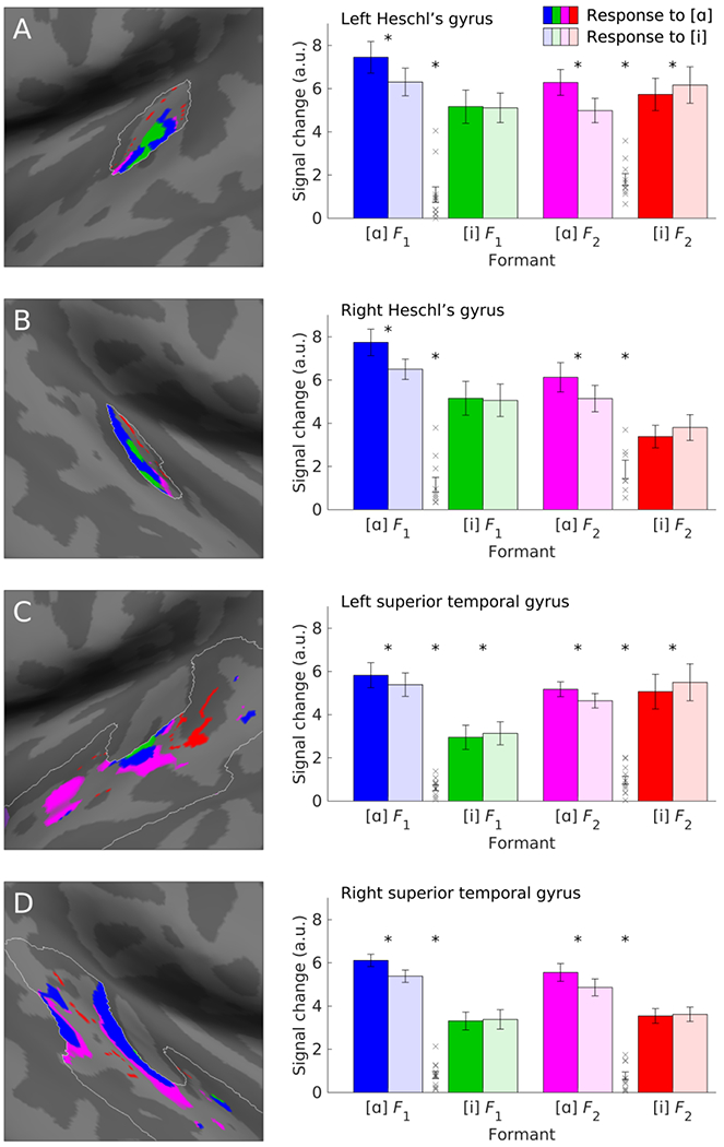
Responses to vowels [ɑ] and [i] in each formant band within each anatomical ROI. Images show voxels that defined each formant band within each anatomical ROI in one representative participant, i.e. voxels that were tonotopic (amplitude F > 3.03), with a best frequency within one of the four formant bands, which are color coded to match the bar plots. (A) Responses in left Heschl’s gyrus (HG). (B) Responses in right HG. (C) Responses in the left superior temporal gyrus (STG). (D) Responses in the right STG. Error bars show standard error of the mean. Xs show the distribution of the interaction contrast (ROI-defining vowel by presented vowel, i.e. [ɑ] response in [ɑ]-based ROI minus [i] response in [ɑ]-based ROI minus [ɑ] response in [i]-based ROI plus [i] response in [i]-based ROI). Note that the interaction contrast was positive (consistent with our primary hypothesis) for all participants for both the first and second formants in each anatomical region of interest. Statistical significance is indicated by * (paired t-test, p < 0.05).

Mean signal changes to the vowels [ɑ] and [i] in each formant-based ROI were then compared (Figure 3, right). There was a significant interaction of ROI-defining vowel by presented vowel (likelihood ratio test statistic = 8.91; p = 0.005). This interaction was driven by significantly greater signal change for [ɑ] (6.28 mean ± 0.31 sd arbitrary units) than [i] (5.40 ± 0.31) in regions based on [ɑ] formants (likelihood ratio test statistic = 16.67; p < 0.001), and numerically greater signal change for [i] (4.48 ± 0.32) than [ɑ] (4.30 ± 0.32) in regions based on [i] formants (likelihood ratio test statistic = 0.39; p = 0.47), confirming the hypothesis that the vowels [ɑ] and [i] would differentially activate tonotopic regions with best frequencies corresponding to their specific formants. The larger difference between responses to the two vowels in the [ɑ] formant bands may reflect the greater energy differences between the vowel stimuli in these bands (Figure 1B).

None of the higher level interactions involving ROI-defining vowel and presented vowel approached significance (all p ≥ 0.43), suggesting that the interaction of ROI-defining vowel by presented vowel was not modulated by or specific to either region, hemisphere, or formant number. As shown in Figure 3, the vowels [ɑ] and [i] differentially activated tonotopic regions with best frequencies corresponding to their specific formants in both HG and the STG, in both hemispheres, and in regions corresponding to the first and second formants. The effect size of the key interaction for each region, hemisphere and formant is shown in Table 3.

Table 3.

Effect size of key interaction for each region of interest and formant

Formant	F1	F2
Left HG	0.88	2.07
Right HG	1.01	1.65
Left STG	1.31	1.53
Right STG	1.42	1.27

Cohen’s d_z for the interaction of ROI-defining vowel by presented vowel.

Because ROIs were defined with an arbitrary two-voxel extent threshold, we checked whether similar results were obtained with other possible thresholds (i.e., no threshold, 5 voxels, 10 voxels). The key interaction of ROI-defining vowel by presented vowel was highly significant regardless of the threshold. Because most participants had few voxels in the [i] F₂ HG ROIs (see Table 2), higher level interactions could not be examined when the extent threshold was increased.

3.4. Prediction of vowel identity from neural data

The identity of untrained blocks of vowels was predicted with mean accuracy of 73.2 ± 9.7% by LDA using signal change from formant-based ROIs, which was significantly better than chance (|t₍₁₁₎| = 8.30; p < 0.001) (Figure 4).

Figure 4.

Classification of untrained vowel blocks on the basis of mean signal change in formant-based regions of interest. HG = Heschl’s gyrus; STG = superior temporal gyrus; L = left; R = right; F₁ = first formant; F₂ = second formant.

In contrast, classifiers based on the two null permutations performed less well. The classifier based on the first null permutation—contiguous but misplaced formants of the same widths—performed with mean accuracy of 63.1 ± 11.5%, which was better than chance (|t₍₁₁₎| = 3.92; p = 0.002), but inferior to the real classifier (|t₍₁₁₎| = 3.12; p = 0.010). The classifiers based on the second null permutation—randomly permuted noncontiguous frequency bands—had a mean accuracy of 64.0 ± 4.8% (standard deviation across participants), which was better than chance (|t₍₁₁₎| = 10.01; p < 0.001). However, the performance of the real classifier fell outside the maximum of the distribution of 1000 permutations (p < 0.001). It is not surprising that null classifiers performed better than chance, since voxels within formant bands were included in these classifiers (albeit not organized optimally), and moreover there are spectral differences between the vowels in frequency ranges other than their formants.

Accuracy did not differ between classifiers based on HG (mean = 69.4 ± 13.2%) and classifiers based on the STG (mean = 70.1 ± 9.8%; |t₍₁₁₎| = 0.19; p = 0.86), nor did it differ between classifiers based on left hemisphere ROIs (mean = 70.6 ± 7.8%) and classifiers based on right hemisphere ROIs (mean = 67.1 ± 12.6%; |t₍₁₁₎| = 0.80; p = 0.44), nor did it differ between classifiers based on F₁ formant bands (mean = 69.3 ± 10.8%) and classifiers based on F₂ formant bands (mean = 68.8 ± 9.8%; |t₍₁₁₎| = 0.17; p = 0.87) (Figure 4).

4. Discussion

The aim of this study was to determine whether vowels are encoded in tonotopic auditory regions in terms of their formants. We found strong evidence that this is the case. In particular, the significant interaction of ROI-defining vowel by presented vowel indicates that [ɑ] and [i] differentially activated tonotopic regions with best frequencies corresponding to their specific formants. This pattern held independently in HG and the STG, in the left and right hemispheres, and in regions corresponding to first and second formants (F₁, F₂). Classifiers trained on mean signal in each formant-based ROI were able to predict the identity of held-out vowel blocks approximately 73% of the time, and performance was almost as good when restricted by region, hemisphere, or formant number.

The cortical encoding of vowel formants in tonotopic regions is broadly consistent with animal studies of primary auditory cortex. Vowel spectra are represented tonotopically in the auditory nerve (Sachs and Young, 1979), and this tonotopy is maintained in the ascending auditory pathways. Electrophysiological studies have shown that population responses to vowels in neurons defined by their best frequencies at least coarsely reflect the spectra of distinct vowels in ferrets (Versnel and Shamma, 1998; Mesgarani et al., 2008; Walker et al., 2011), cats (Qin et al., 2008) and rats (Honey and Schnupp, 2015). Similarly, animal vocalizations (Wang et al., 1995; Qin et al., 2008) and the formant transitions that cue consonant place of articulation (Steinschneider et al., 1995; Engineer et al., 2008; Steinschneider and Fishman, 2011) are also represented in tonotopic auditory cortex according to their spectral content. However, encoding of vowel formant frequencies in primary auditory cortex is not always straightforwardly predictable from neural responses to simpler sounds. For instance, Versnel and Shamma (1998) showed that spike counts reflected the slopes in the spectra of different vowels quite well in the 1400 to 2000 Hz range, but were fairly flat, failing to follow spectral details of vowels, in the 2000 to 2800 Hz region. Some researchers have proposed that primary auditory cortex does not encode formants veridically, but rather encodes some derivative such as the difference between F₁ and F₂ (Ohl and Scheich, 1997).

The cortical encoding of vowels in terms of spectral information, and ability to reconstruct this spectral information from functional MRI data, is consistent with previous functional imaging studies of cortical encoding of natural sounds in humans (Moerel et al., 2012, 2013; Santoro et al., 2014, 2017). With regard to vowels specifically, MEG studies have shown differences between vowels in equivalent current dipole localization of the N1m component (Diesch and Luce 1997; Mäkelä et al., 2003; Obleser et al., 2003, 2004; Shestakova et al., 2004; Scharinger et al., 2011, 2012). These studies have shown that vowel pairs that are more dissimilar in F₁/F₂ space, or that differ by more distinctive features, generally show larger Euclidean distances between their dipole locations (Manca and Grimaldi, 2016). However the specific orientations of differences in dipole locations in relation to formant frequencies have been inconsistent across studies (Manca and Grimaldi, 2016). This may reflect the fact that single dipoles are used to model complex patterns of activity that involve the representation of multiple formants on multiple tonotopic gradients, which may be oriented in idiosyncratic ways according to individual anatomy of Heschl’s gyrus and other tonotopically organized regions.

Functional MRI has better spatial resolution that MEG and should in principle be able to resolve differences between multiple formants on multiple tonotopic gradients. However, activation differences have almost never been reported in univariate subtraction-based analyses (e.g. Formisano et al., 2008; Obleser et al., 2010). Only one study to our knowledge has reported this kind of topographic segregation of vowel responses, with back vowels yielding anterior activation relative to front vowels in anterior temporal cortex (Obleser et al., 2006). However this relative orientation is inconsistent with MEG findings (Obleser et al., 2004; Scharinger et al., 2011), and the finding was not replicated in a later functional MRI study from the same group (Obleser et al., 2010). Probably the main reason that we were able to show robust univariate differences between vowels in the present study was that we did not attempt a whole-brain analysis, but rather used tonotopic mapping to identify hypothesis-driven ROIs in each individual participant.

The imaging and electrocorticography studies that have demonstrated neural discrimination between vowels in humans have done so on the basis of distributed representations (Formisano et al., 2008; Obleser et al., 2010; Bonte et al., 2014; Mesgarani et al., 2014). When the patterns of voxels or electrodes contributing to these classifications have been reported, they have appeared to be spatially dispersed (Mesgarani et al., 2014 (supplementary material); Zhang et al., 2016). However the accuracy with which we could reconstruct vowel identity in the present study compares favorably to discrimination between vowels in several neuroimaging studies that have done so using multi-voxel pattern analysis of distributed patterns of activity. For instance, Formisano et al. (2008) reported classification accuracies of 65% or 66% in discriminating [a] from [i] in two different circumstances; see also Obleser et al. (2010), Bonte et al. (2014) and Zhang et al. (2016) for similar findings. This raises the question of to what extent discrimination in these studies is driven by voxels in tonotopic regions. It is apparent from electrocorticography studies that the electrodes responsible for encoding classes of vowels have spectrotemporal receptive fields corresponding to the vowel spectra (Mesgarani et al., 2014). This is even clearer in single unit animal data (Mesgarani et al., 2008). Therefore it is quite likely that responses in tonotopic regions make a major contribution to reconstruction of vowel identity in human imaging studies too.

Our study had several noteworthy limitations. First, we did not control the stimulus presentation level, instead presenting stimuli at individualized levels such that the frequency sweeps and vowels could be comfortably heard over the loud background noise of the scanner. Versnel and Shamma (1998) showed that in ferrets, cortical responses to vowels were fairly consistent over a 20-dB range. However there were some cases where responses to vowels changed markedly as a function of level. It will be important to investigate the level dependence of cortical responses to vowels in humans.

Second, we characterized each tonotopic voxel in terms of a single best frequency based on Fourier analysis of bandpass-swept nonverbal human vocalizations. However, recent functional imaging studies have shown that the spectral tuning profiles of voxels are much more complex than this (Moerel et al., 2013, 2015; Allen et al., 2017, 2018). Many voxels are sensitive to multiple frequency peaks, sometimes but not always harmonically related to one another, and even voxels with single peaks vary in the width of their tuning curves, and in the presence or absence of inhibitory sidebands (Moerel et al., 2013). It would be worthwhile to investigate whether a richer characterization of voxels’ spectral receptive fields would permit more accurate reconstruction of vowel identity (Versnel and Shamma, 1998). Another consideration is that spectral tuning can depend on context. While tonotopic maps derived from pure tones and natural sounds (such as the nonverbal human vocalizations we used) are fundamentally similar (Moerel et al., 2012), tonotopy can arise from selective attention alone (Da Costa et al., 2013; Riecke et al., 2017; Dick et al., 2017), demonstrating its contextual flexibility. A study of ferrets showed rapid plasticity of spectrotemporal receptive fields such that neurons’ best frequencies came to be centered on the stimulus frequency relevant for a food reward task (Fritz et al., 2003). It is intriguing to speculate that such shifts might underlie processes such as talker normalization.

Third, although the interaction of ROI-defining vowel by presented vowel was highly significant, it was not the case that the patterns of signal change in the formant-based ROIs (Figure 3) closely resembled the spectra of the presented vowels (Figure 1). In particular, all ROIs showed strong positive responses to both vowels. One relevant consideration is that all vowels contain broadband energy across the frequency spectrum, not just in the peaks that define their formants. Furthermore, as just described, the complexity of voxels’ spectral tuning profiles might imply that most voxels would respond to some extent to any vowel. Finally, the spatial resolution of fMRI may lead to conflation of finer grained vowel-specific responses.

Fourth, although we confirmed our hypothesis that vowels would differentially activate tonotopic regions that represent their formants, we cannot rule out that linguistic shaping or processing of the input may also have taken place. There is compelling evidence that speech perception depends on higher order encoding such as the differences between formant frequencies rather than their absolute values (Potter and Steinberg, 1950; Syrdal and Gopal, 1986; Ohl and Scheich, 1997; Mesgarani et al., 2014). Moreover, speech perception is warped by linguistic experience such that perceptual space shrinks in the region of category prototypes and expands closer to category boundaries (Kuhl, 1991; Iverson and Kuhl, 1995). Our experiment was not designed to investigate these types of effects, since we deliberately used vowels that were maximally distinct in terms of their formants in order to maximize our ability to detect tonotopic representation. The basic tonotopic organization that we documented certainly does not exclude that there is also higher level more abstract encoding of phonemic representations in HG and the STG. Future studies will hopefully be able to build upon the findings of the present study to investigate linguistic processing of speech sounds beyond their representation in terms of the basic auditory organizing principle of tonotopy.

In conclusion, this study showed that the identities of vowels can be reliably predicted from cortical tonotopic representations of their formants. This suggests that tonotopic organization plays a fundamental role in the cortical encoding of vowel sounds and may act as a scaffold for further linguistic processing.

References

- Allen EJ, Burton PC, Olman CA, Oxenham AJ, 2017. Representations of pitch and timbre variation in human auditory cortex. J. Neurosci. 37, 1284–1293. [DOI] [PMC free article] [PubMed] [Google Scholar]
- Allen EJ, Moerel M, Lage-Castellanos A, De Martino F, Formisano E, Oxenham AJ, 2018. Encoding of natural timbre dimensions in human auditory cortex. NeuroImage 166, 60–70. [DOI] [PMC free article] [PubMed] [Google Scholar]
- American Speech-Language-Hearing Association, 1997. Guidelines for audiologic screening. doi: 10.1044/policy.GL1997-00199. [DOI] [Google Scholar]
- Arsenault JS, Buchsbaum BR, 2015. Distributed neural representations of phonological features during speech perception. J. Neurosci. 35, 634–642. [DOI] [PMC free article] [PubMed] [Google Scholar]
- Bates D, Mächler M, Bolker B, Walker S, 2015. Fitting linear mixed-effects models using lme4. J. Stat. Softw. 67, 1–48. [Google Scholar]
- Belin P, Fillion-Bilodeau S, Gosselin F 2008. The Montreal Affective Voices: a validated set of nonverbal affect bursts for research on auditory affective processing. Behav. Res. Methods 40, 531–539. [DOI] [PubMed] [Google Scholar]
- Bidelman GM, Moreno S, Alain C, 2013. Tracing the emergence of categorical speech perception in the human auditory system. NeuroImage 79, 201–212. [DOI] [PubMed] [Google Scholar]
- Boersma P 2001. Praat, a system for doing phonetics by computer. Glot International 5(9/10), 341–345. [Google Scholar]
- Bonte M, Hausfeld L, Scharke W, Valente G, Formisano E, 2014. Task-dependent decoding of speaker and vowel identity from auditory cortical response patterns. J. Neurosci. 34, 4548–4557. [DOI] [PMC free article] [PubMed] [Google Scholar]
- Chan AM, Dykstra AR, Jayaram V, Leonard MK, Travis KE, Gygi B, Baker JM, Eskandar E, Hochberg LR, Halgren E, Cash SS, 2014. Speech-specific tuning of neurons in human superior temporal gyrus. Cereb Cortex 24, 2679–2693. [DOI] [PMC free article] [PubMed] [Google Scholar]
- Chang EF, Rieger JW, Johnson K, Berger MS, Barbaro NM, Knight RT, 2010. Categorical speech representation in human superior temporal gyrus. Nat. Neurosci. 13, 1428–1433. [DOI] [PMC free article] [PubMed] [Google Scholar]
- Cox RW, 1996. AFNI: software for analysis and visualization of functional magnetic resonance neuroimages. Comput. Biomed. Res. 29, 162–173. [DOI] [PubMed] [Google Scholar]
- Da Costa S, van der Zwaag W, Marques JP, Frackowiak RSJ, Clarke S, Saenz M, 2011. Human primary auditory cortex follows the shape of Heschl’s gyrus. J. Neurosci. 31, 14067–14075. [DOI] [PMC free article] [PubMed] [Google Scholar]
- Da Costa S, van der Zwaag W, Miller LM, Clarke S, Saenz M, 2013. Tuning in to sound: frequency-selective attentional filter in human primary auditory cortex. J. Neurosci. 33, 1858–1863. [DOI] [PMC free article] [PubMed] [Google Scholar]
- Dale AM, Fischl B, Sereno MI, 1999. Cortical surface-based analysis. I. Segmentation and surface reconstruction. NeuroImage 9, 179–194. [DOI] [PubMed] [Google Scholar]
- De Martino F, Moerel M, Xu J, van de Moortele P-F, Ugurbil K, Goebel R, Yacoub E, Formisano E, 2015. High-resolution mapping of myeloarchitecture in vivo: localization of auditory areas in the human brain. Cereb. Cortex 25, 3394–3405. [DOI] [PMC free article] [PubMed] [Google Scholar]
- Desikan RS, Ségonne F, Fischl B, Quinn BT, Dickerson BC, Blacker D, Buckner RL, Dale AM, Maguire RP, Hyman BT, Albert MS, Killiany RJ, 2006. An automated labeling system for subdividing the human cerebral cortex on MRI scans into gyral based regions of interest. NeuroImage 31, 968–980. [DOI] [PubMed] [Google Scholar]
- Dick F, Tierney AT, Lutti A, Josephs O, Sereno MI, Weiskopf N, 2012. In vivo functional and myeloarchitectonic mapping of human primary auditory areas. J. Neurosci. 32, 16095–16105. [DOI] [PMC free article] [PubMed] [Google Scholar]
- Dick FK, Lehet MI, Callaghan MF, Keller TA, Sereno MI, Holt LL, 2017. Extensive tonotopic mapping across auditory cortex is recapitulated by spectrally directed attention and systematically related to cortical myeloarchitecture. J. Neurosci. 37, 12187–12201. [DOI] [PMC free article] [PubMed] [Google Scholar]
- Diesch E, Luce T, 1997. Magnetic fields elicited by tones and vowel formants reveal tonotopy and nonlinear summation of cortical activation. Psychophysiology 34, 501–510. [DOI] [PubMed] [Google Scholar]
- Engineer CT, Perez CA, Chen YH, Carraway RS, Reed AC, Shetake JA, Jakkamsetti V, Chang KQ, Kilgard MP, 2008. Cortical activity patterns predict speech discrimination ability. Nat. Neurosci. 11, 603–608. [DOI] [PMC free article] [PubMed] [Google Scholar]
- Evans S, Davis MH, 2015. Hierarchical organization of auditory and motor representations in speech perception: evidence from searchlight similarity analysis. Cereb. Cortex 25, 4772–4788. [DOI] [PMC free article] [PubMed] [Google Scholar]
- Faraway JJ, 2016. Extending the linear model with R: generalized linear, mixed effects and nonparametric regression models, second ed. CRC press, Boca Raton. [Google Scholar]
- Fischl B, van der Kouwe A, Destrieux C, Halgren E, Ségonne F, Salat DH, Busa E, Seidman LJ, Goldstein J, Kennedy D, Caviness V, Makris N, Rosen B, Dale AM, 2004. Automatically parcellating the human cerebral cortex. Cereb. Cortex 14, 11–22. [DOI] [PubMed] [Google Scholar]
- Formisano E, De Martino F, Bonte M, Goebel R, 2008. “Who” is saying “what”? Brain-based decoding of human voice and speech. Science 322, 970–973. [DOI] [PubMed] [Google Scholar]
- Fritz J, Shamma S, Elhilali M, Klein D, 2003. Rapid task-related plasticity of spectrotemporal receptive fields in primary auditory cortex. Nat. Neurosci. 6, 1216–1223. [DOI] [PubMed] [Google Scholar]
- Honey C, Schnupp J, 2015. Neural resolution of formant frequencies in the primary auditory cortex of rats. PLoS One 10, e0134078. [DOI] [PMC free article] [PubMed] [Google Scholar]
- Humphries C, Liebenthal E, Binder JR, 2010. Tonotopic organization of human auditory cortex. NeuroImage 50, 1202–1211. [DOI] [PMC free article] [PubMed] [Google Scholar]
- Iverson P, Kuhl PK, 1995. Mapping the perceptual magnet effect for speech using signal detection theory and multidimensional scaling. J. Acoust. Soc. Am. 97, 553–562. [DOI] [PubMed] [Google Scholar]
- Kilian-Hütten N, Valente G, Vroomen J, Formisano E, 2011. Auditory cortex encodes the perceptual interpretation of ambiguous sound. J. Neurosci. 31, 1715–1720. [DOI] [PMC free article] [PubMed] [Google Scholar]
- Kuhl PK, 1991. Human adults and human infants show a “perceptual magnet effect” for the prototypes of speech categories, monkeys do not. Percept. Psychophys. 50, 93–107. [DOI] [PubMed] [Google Scholar]
- Leonard MK, Baud MO, Sjerps MJ, Chang EF, 2016. Perceptual restoration of masked speech in human cortex. Nat. Commun. 7, 13619. [DOI] [PMC free article] [PubMed] [Google Scholar]
- Mäkelä AM, Alku P, Tiitinen H, 2003. The auditory N1m reveals the left-hemispheric representation of vowel identity in humans. Neurosci. Lett. 353, 111–114. [DOI] [PubMed] [Google Scholar]
- Manca AD, Grimaldi M, 2016. Vowels and consonants in the brain: evidence from magnetoencephalographic studies on the N1m in normal-hearing listeners. Front. Psychol 7. [DOI] [PMC free article] [PubMed] [Google Scholar]
- Mesgarani N, Cheung C, Johnson K, Chang EF, 2014. Phonetic feature encoding in human superior temporal gyrus. Science 343, 1006–1010. [DOI] [PMC free article] [PubMed] [Google Scholar]
- Mesgarani N, David SV, Fritz JB, Shamma SA, 2008. Phoneme representation and classification in primary auditory cortex. J. Acoust. Soc. Am. 123, 899–909. [DOI] [PubMed] [Google Scholar]
- Moerel M, De Martino F, Santoro R, Yacoub E, Formisano E, 2015. Representation of pitch chroma by multi-peak spectral tuning in human auditory cortex. NeuroImage 106, 161–169. [DOI] [PMC free article] [PubMed] [Google Scholar]
- Moerel M, Martino FD, Formisano E, 2012. Processing of natural sounds in human auditory cortex: tonotopy, spectral tuning, and relation to voice sensitivity. J. Neurosci. 32, 14205–14216. [DOI] [PMC free article] [PubMed] [Google Scholar]
- Moerel M, Martino FD, Santoro R, Ugurbil K, Goebel R, Yacoub E, Formisano E, 2013. Processing of natural sounds: characterization of multipeak spectral tuning in human auditory cortex. J. Neurosci. 33, 11888–11898. [DOI] [PMC free article] [PubMed] [Google Scholar]
- Moses DA, Mesgarani N, Leonard MK, Chang EF, 2016. Neural speech recognition: continuous phoneme decoding using spatiotemporal representations of human cortical activity. J. Neural Eng. 13, 056004. [DOI] [PMC free article] [PubMed] [Google Scholar]
- Obleser J, Boecker H, Drzezga A, Haslinger B, Hennenlotter A, Roettinger M, Eulitz C, Rauschecker JP, 2006. Vowel sound extraction in anterior superior temporal cortex. Hum. Brain Mapp. 27, 562–571. [DOI] [PMC free article] [PubMed] [Google Scholar]
- Obleser J, Elbert T, Lahiri A, Eulitz C, 2003. Cortical representation of vowels reflects acoustic dissimilarity determined by formant frequencies. Cogn. Brain Res. 15, 207–213. [DOI] [PubMed] [Google Scholar]
- Obleser J, Lahiri A, Eulitz C, 2004. Magnetic brain response mirrors extraction of phonological features from spoken vowels. J. Cogn. Neurosci. 16, 31–39. [DOI] [PubMed] [Google Scholar]
- Obleser J, Leaver AM, Vanmeter J, Rauschecker JP, 2010. Segregation of vowels and consonants in human auditory cortex: evidence for distributed hierarchical organization. Front. Psychol. 1, 232. [DOI] [PMC free article] [PubMed] [Google Scholar]
- Ohl FW, Scheich H, 1997. Orderly cortical representation of vowels based on formant interaction. Proc. Natl. Acad. Sci. U. S. A. 94, 9440–9444. [DOI] [PMC free article] [PubMed] [Google Scholar]
- Pasley BN, David SV, Mesgarani N, Flinker A, Shamma SA, Crone NE, Knight RT, Chang EF, 2012. Reconstructing speech from human auditory cortex. PLoS Biology 10, e1001251. [DOI] [PMC free article] [PubMed] [Google Scholar]
- Peterson GE, Barney HL, 1952. Control methods used in a study of the vowels. J. Acoust. Soc. Am. 24, 175–184. [Google Scholar]
- Potter RK, Steinberg JC, 1950. Toward the specification of speech. J. Acoust. Soc. Am. 22, 807–820. [Google Scholar]
- Qin L, Wang JY, Sato Y, 2008. Representations of cat meows and human vowels in the primary auditory cortex of awake cats. J. Neurophysiol. 99, 2305–2319. [DOI] [PubMed] [Google Scholar]
- R Core Team, 2018. R: A language and environment for statistical computing R Foundation for Statistical Computing, Vienna, Austria: https://www.r-project.org. [Google Scholar]
- Riecke L, Peters JC, Valente G, Kemper VG, Formisano E, Sorger B, 2016. Frequency-selective attention in auditory scenes recruits frequency representations throughout human superior temporal cortex. Cereb. Cortex 27, 3002–3014. [DOI] [PubMed] [Google Scholar]
- Sachs MB, Young ED, 1979. Encoding of steady-state vowels in the auditory nerve: Representation in terms of discharge rate. J. Acoust. Soc. Am. 66, 470–479. [DOI] [PubMed] [Google Scholar]
- Saenz M, Langers DRM, 2013. Tonotopic mapping of human auditory cortex. Hear. Res. 307, 42–52. [DOI] [PubMed] [Google Scholar]
- Santoro R, Moerel M, De Martino F, Goebel R, Ugurbil K, Yacoub E, Formisano E, 2014. Encoding of natural sounds at multiple spectral and temporal resolutions in the human auditory cortex. PLoS Comput Biol 10, e1003412. [DOI] [PMC free article] [PubMed] [Google Scholar]
- Scharinger M, Idsardi WJ, Poe S, 2011. A comprehensive three-dimensional cortical map of vowel space. J. Cogn. Neurosci. 23, 3972–3982. [DOI] [PubMed] [Google Scholar]
- Scharinger M, Monahan PJ, Idsardi WJ, 2012. Asymmetries in the processing of vowel height. J. Speech Lang. Hear. Res. 55, 903–918. [DOI] [PubMed] [Google Scholar]
- Sereno MI, Dale AM, Reppas JB, Kwong KK, Belliveau JW, Brady TJ, Rosen BR, Tootell RB, 1995. Borders of multiple visual areas in humans revealed by functional magnetic resonance imaging. Science 268, 889–893. [DOI] [PubMed] [Google Scholar]
- Shestakova A, Brattico E, Soloviev A, Klucharev V, Huotilainen M, 2004. Orderly cortical representation of vowel categories presented by multiple exemplars. Cogn. Brain Res. 21, 342–350. [DOI] [PubMed] [Google Scholar]
- Steinschneider M, Fishman YI, 2011. Enhanced physiologic discriminability of stop consonants with prolonged formant transitions in awake monkeys based on the tonotopic organization of primary auditory cortex. Hear. Res. 271, 103–114. [DOI] [PMC free article] [PubMed] [Google Scholar]
- Steinschneider M, Reser D, Schroeder CE, Arezzo JC, 1995. Tonotopic organization of responses reflecting stop consonant place of articulation in primary auditory cortex (A1) of the monkey. Brain Res. 674, 147–152. [DOI] [PubMed] [Google Scholar]
- Striem-Amit E, Hertz U, Amedi A, 2011. Extensive cochleotopic mapping of human auditory cortical fields obtained with phase-encoding FMRI. PLoS One 6, e17832. [DOI] [PMC free article] [PubMed] [Google Scholar]
- Syrdal AK, Gopal HS, 1986. A perceptual model of vowel recognition based on the auditory representation of American English vowels. J. Acoust. Soc. Am. 79, 1086–1100. [DOI] [PubMed] [Google Scholar]
- Talavage TM, Sereno MI, Melcher JR, Ledden PJ, Rosen BR, Dale AM, 2004. Tonotopic organization in human auditory cortex revealed by progressions of frequency sensitivity. J. Neurophysiol. 91, 1282–1296. [DOI] [PubMed] [Google Scholar]
- Versnel H, Shamma SA, 1998. Spectral-ripple representation of steady-state vowels in primary auditory cortex. J. Acoust. Soc. Am. 103, 2502–2514. [DOI] [PubMed] [Google Scholar]
- Walker KMM, Bizley JK, King AJ, Schnupp JWH, 2011. Multiplexed and robust representations of sound features in auditory cortex. J. Neurosci. 31, 14565–14576. [DOI] [PMC free article] [PubMed] [Google Scholar]
- Wang X, Merzenich MM, Beitel R, Schreiner CE, 1995. Representation of a species-specific vocalization in the primary auditory cortex of the common marmoset: temporal and spectral characteristics. J. Neurophysiol. 74, 2685–2706. [DOI] [PubMed] [Google Scholar]
- Woods DL, Stecker GC, Rinne T, Herron TJ, Cate AD, Yund EW, Liao I, Kang X, 2009. Functional maps of human auditory cortex: effects of acoustic features and attention. PLoS One 4, e5183. [DOI] [PMC free article] [PubMed] [Google Scholar]
- Worsley KJ, Liao CH, Aston J, Petre V, Duncan GH, Morales F, Evans AC, 2002. A general statistical analysis for fMRI data. NeuroImage 15, 1–15. [DOI] [PubMed] [Google Scholar]
- Young ED, 2008. Neural representation of spectral and temporal information in speech. Philos. Trans. Royal Soc. B 363, 923–945. [DOI] [PMC free article] [PubMed] [Google Scholar]
- Zhang Q, Hu X, Luo H, Li J, Zhang X, Zhang B, 2016. Deciphering phonemes from syllables in blood oxygenation level-dependent signals in human superior temporal gyrus. Eur. J. Neurosci. 43, 773–781. [DOI] [PubMed] [Google Scholar]