Figure 5.

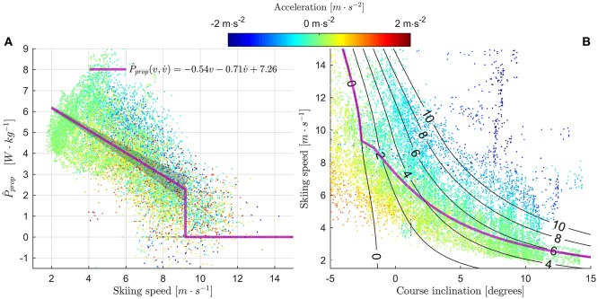
(A) Propulsive power (normalized to body mass) was approximately linearly related to skiing speed (v) and acceleration ($\dot{v}$) in the skiing direction. Data from all athletes are included in the figure, and data points are color coded by $\dot{v}$, as indicated by the colorbar above the figure. The magenta-colored line is the least squares regression fit to samples where the athlete was not in the tucked position. The shaded region indicates the measurement error (SD), see Figure 7 for details. (B) Plot of skiing speed vs. the course inclination. Data points are color coded as in panel (A). The black lines indicate constant propulsive power (in W·kg⁻¹), assuming constant skiing speed ($\dot{v}$ = 0). The magenta line shows the steady state skiing speed obtained from the regression line in (A). It was defined as the real root of the 3rd degree polynomial obtained by replacing P_prop with P_prop(v,$\dot{v}$) in Equation 1, and assuming a constant drag area of 0.55 m² and average body mass 77.1 kg. For v > 9 m·s⁻¹ the line was defined to follow the zero-P_prop iso-line. The figure clearly shows that data points where $\dot{v}$ ≈ 0 (green color) are distributed close to the steady-state speed line, as expected. Data points below the steady-state line have $\dot{v}$ > 0 (red), and data points above the line have $\dot{v}$ < 0. This is mainly attributed to the athletes' inertias.