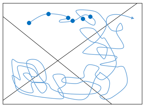
Figure 6.

The basis for “decorrelation analysis” [32]. From a continuous trajectory (blue curve), configurations can be extracted at equally spaced time points (filled circles) with each such configuration categorized as belonging to one of a set of arbitrary states (delineated by straight black lines). If the configurations are statistically independent – if they are sufficiently decorrelated – then their statistical behavior will match that predicted by a multinomial distribution consistent with the trajectory’s fractional populations in each state. A range of time-spacings can be analyzed to determined if and when such independence occurs.