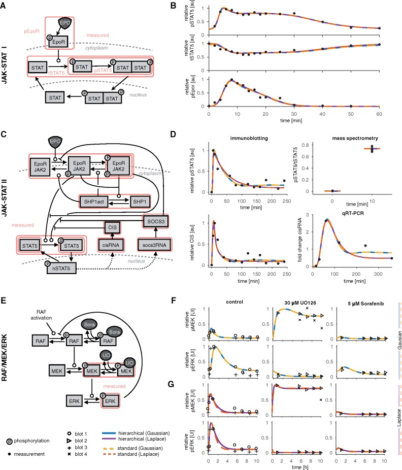
Fig. 3.

Models and experimental data. (A, B) JAK-STAT I. (A) Illustration of the model according to Swameye et al. (2003). Arrows represent biochemical reactions, and the observables of the model used are highlighted by boxes. (B) Experimental data and fitted trajectories for the best parameter found with multi-start local optimization with 100 starts. The results are shown for the standard (dotted lines) and hierarchical (solid lines) approach for optimization for Gaussian and Laplace noise. (C, D) JAK-STAT II. (C) Illustration of the model according to Bachmann et al. (2011). (D) Experimental data and fitted trajectories for the best parameter found with multi-start local optimization for 100 and 200 starts for Gaussian and Laplace noise, respectively. 33 out of 541 data points are shown. (E–G) RAF/MEK/ERK. (E) Illustration of the model according to Fiedler et al. (2016). (F, G) Experimental data and fitted trajectories for the best parameter found with multi-start local optimization for 500 and 1000 starts for Gaussian and Laplace noise, respectively. Different markers indicate the different blots. The data is scaled according to the estimated scaling parameters, yielding different visualizations for different parameters, as obtained with the Gaussian and the Laplace noise assumption. (F) Fitted trajectories for Gaussian noise for the standard (dotted line) and hierarchical (solid line) approach for optimization. (G) Fitted trajectories for Laplace noise