A LAGRANGIAN FORMULATION FOR STATISTICAL FLUID REGISTRATION

Abstract

We defined a new statistical fluid registration method with Lagrangian mechanics. Although several authors have suggested that empirical statistics on brain variation should be incorporated into the registration problem, few algorithms have included this information and instead use regularizers that guarantee diffeomorphic mappings. Here we combine the advantages of a large-deformation fluid matching approach with empirical statistics on population variability in anatomy. We reformulated the Riemannian fluid algorithm developed in [4], and used a Lagrangian framework to incorporate 0^th and 1^rst order statistics in the regularization process. 92 2D midline corpus callosum traces from a twin MRI database were fluidly registered using the non-statistical version of the algorithm (algorithm 0), giving initial vector fields and deformation tensors. Covariance matrices were computed for both distributions and incorporated either separately (algorithm 1 and algorithm 2) or together (algorithm 3) in the registration. We computed heritability maps and two vector and tensor-based distances to compare the power and the robustness of the algorithms.

1. INTRODUCTION

Nonlinear image registration is widely used in the medical field with numerous applications ranging from real time matching in surgical procedures, to alignment of functional and structural images, and multi-modal atlas construction. Depending on their use, these methods have different requirements in terms of efficiency and precision. For instance, a precise registration is typically needed in computational morphometry to map the influence of disease, genetics or normal development throughout the brain, while robust methods are needed for atlas-based segmentation in more clinically oriented applications.

Warping one image or volume onto another requires the definition of a similarity term (also called the cost function) to compare information in the two images, such as a distance between common anatomical or stereotactic landmarks, or intensity-based measures over the whole image, e.g., the squared intensity difference (L²-norm), cross-correlation or metrics derived from information theory [7]. If driven by a cost function only, irregularities would appear in the deformation. A regularizer is added, to enforce desirable properties, such as smoothness, invertibility and inverse-consistency [5]. These criteria can be enforced by using equations from elastic or fluid mechanics [2, 8, 3, 12] or through other non-physical regularization models, such as Gaussian filtering [22] or the optimization of geodesic trajectories [18, 9].

As registration is guided by information in two overlaid images, and one scalar value per voxel is used to generate maps of 2D or 3D vectors, finding a unique solution is impossible. Some prior knowledge regarding the dataset can therefore be valuable to ensure a meaningful deformation. To incorporate empirical information, earlier studies focused on (1) principal component analysis of intra-subject registration fields [11], (2) estimation of covariance structures of the deformations from a training set of examples [6] or (3) spectral methods, in which the deformations were projected onto the eigenfunctions of the operator governing the deformation, and statistics of the resulting coefficients were used to infer anatomical abnormalities [13]. In all these works, one important question is: which statistical information is most reliable for estimating deformations, and how can they be included in a registration algorithm?

In this paper, we used 0th- and 1st-order spatial statistics on the deformation within a fluid algorithm, i.e., the mean and covariance of the displacement fields and of the strain tensors. A fluid formulation was used because elastic media can only be deformed up to a point, after which the restoring forces become too strong and the medium ceases to obey the linear elastic equation. Fluid registration, however, guarantees that transformations remain diffeomorphic even for large deformations.

Statistics on the deformation tensors Σ (where Σ = J^T J, where J = (Id + ∇u) is the jacobian matrix and $\overrightarrow{u}$ is the displacement) were previously incorporated in the regularization of an elastic algorithm in [20] using a Riemannian framework. The authors proposed a regularizer, which contains the covariance of the Σ and penalizes these full deformation tensors. These matrices represent anisotropic deformations (i.e., ones with a preferred direction locally) as well as volumetric excesses and deficits. As the Σ’s are symmetric positive-definite matrices and form a cone in the space of 3×3 real-valued matrices, standard Euclidean operations are not accurate in the manifold formed by the Σ. The Log-Euclidean framework [1] solves this problem and allows simple computations to be made intrinsically on this manifold. The isotropic version of the Riemannian regularizer was derived in closed form and used for elastic registration in [20]. In [4], we extended this work to the fluid case, regularizing the rate of strain $\log ({(\nabla \overrightarrow{v}+Id)}^T(\nabla \overrightarrow{v}+Id))$ through the velocity $v(v=\frac{du}{dt})$ (algorithm 0) rather than u.

To include 0^th order spatial statistics, we rewrote algorithm 0 using a Lagrangian structure. In this new framework, the regularizer in [4] is derived from a dissipative Lagrangian, in which we now include statistical information on the data. This new formulation clarifies the meanings of the different terms integrated in the equation in terms of physical entities. We then incorporate empirical statistics, including the covariance of the Σ matrices algorithm 2 and the covariance of the displacement fields algorithm 1 in the dissipation term.

In order to validate and compare the different algorithms, we perform a Tensor-Based Morphometry analysis (see [16]) on 2D corpus callosum traces from 23 monozygotic (MZ) and 23 same-sex dizyotic (DZ) twin pairs. P-value maps, designed to detect known anatomical similarities between twins, illustrate the difference in power between the four versions. Effects were more powerfully detected when 1^rst order statistics were included in the registration process. We also investigated the robustness of these methods by computing two metrics that measure the distance between images. Depending on the definition of the distance used, both algorithms 0 and 1 were shown to be the most robust.

2. DEFINITION OF THE ALGORITHMS

2.1. Previous formulation of the Riemannian Fluid

The Riemannian fluid algorithm regularizes the transformation of one image into another by acting on the rate of strain Σ_v, rather than using traditional fluid equations ( ${\sum }_v={(\nabla \overrightarrow{v}+Id)}^T(\nabla \overrightarrow{v}+Id)$ and v the velocity, or time-derivative of u). In [4], we extended the method proposed in [20] to implement the isotropic Riemannian fluid registration. At each voxel, for each of the time steps Δt, the regularizer and image similarity cost terms were optimized to find the velocity v according to the equation:

$$\frac{d\overrightarrow{v}(\overrightarrow{x},t)}{dt}=\nabla \mathit{\text{Cost}}-\alpha \nabla Re{g}_{\mathit{\text{Riem}}}-v.$$ (1)

v is then integrated over time to find the displacement u. The image similarity criterion Cost is usually defined as the squared intensity difference between the two images I and J, which gives the force:

$$\overrightarrow{F}(\overrightarrow{x},\overrightarrow{u}(\overrightarrow{x},t))=\nabla \mathit{\text{Cost}}(I,J,u)(x)$$ (2)

This cost function will be used throughout the paper, although alternative cost functions, e.g., based on mutual information, could be used instead. The isotropic Riemannian regularizer was as follows:

$$Re{g}_{\mathit{\text{Riem}}}(\overrightarrow{v},t)={\displaystyle \int \frac{\mu }{4}Tr(\log ({\sum }_v^2)+\frac{\lambda }{8}Tr{(\log ({\sum }_v))}^2}$$ (3)

An Isotropic Riemannian Elasticity model can be obtained by replacing Σ_v by Σ (see [20]).

2.2. Lagrangian formulation

A Lagrangian $\mathrm{ℒ}$ expresses the dynamic behavior of a system. We generally take $\mathrm{ℒ}=T-V$ where T and V represent the kinetic and potential energy of the system, respectively. If we call D the dissipation, q_j is the position of the particle j, and ${\dot{q}}_j$ is the velocity at the corresponding position, then the evolution equations of the system are:

$$\frac{d}{dt}(\frac{\partial \mathrm{ℒ}}{\partial {\dot{q}}_j})-(\frac{\partial \mathrm{ℒ}}{\partial q_j})+(\frac{\partial D}{\partial {\dot{q}}_j})=0;$$ (4)

where the dissipation term D quantifies the loss of energy that will allow us to stabilize around the minimum of the potential energy.

2.3. Original algorithm

In the non-statistical version of the algorithm (algorithm 0), we define the different terms as follows:

• Kinetic energy: $T=\frac{1}{2}{\Vert {\dot{q}}_j\Vert }_2^2$

• Potential Energy: V = Cost(q)

• Dissipation: $D=\frac{1}{2}{\Vert {\dot{q}}_j\Vert }_2^2+\alpha \mathit{\text{Reg}}(\dot{q})$

Equation (1) thus becomes:

1. $\frac{d}{dt}(\frac{\partial \mathrm{ℒ}}{\partial {\dot{q}}_j})=\frac{d\overrightarrow{v}(\overrightarrow{q_j},t)}{dt}=\frac{d}{dt}(\frac{\partial }{\partial {\dot{q}}_j}(\frac{1}{2}{\Vert {\dot{q}}_j\Vert }_2^2))$

2. $\frac{\partial \mathrm{ℒ}}{\partial q_j}=\nabla \mathit{\text{Cost}}(I,J,q)$

3. $\frac{\partial D}{\partial {\dot{q}}_j}={\dot{q}}_j+\alpha {\nabla }_{\dot{q}}Re{g}_{\mathit{\text{Riem}}}({\dot{q}}_j)$

This Lagrangian formulation establishes a meaningful interpretation of the fluid system, in which prior statistical information can be included, in particular in the dissipation term.

2.4. Incorporating statistics on the displacement

Algorithm 0 is first run on a dataset to obtain a distribution of vector fields, from which we compute the covariance of the deformation tensors Σ, and the covariance of the displacement fields, $\overrightarrow{u}$. We formulate algorithm 1 by inserting the covariance of the displacements into the velocity term in the dissipation. We replaced the Euclidean norm ‖.‖₂ by a Mahalanobis distance. The first term of the dissipation D becomes

$$D_1={\Vert {\dot{q}}_j\Vert }^2={\dot{q}}_j^{T}co{v}_{q_j}^{(-1)}{\dot{q}}_j$$ (5)

with $co{v}_{q_j}=\frac{1}{N}{\displaystyle {\sum }_i{(q_i-{\overline{q}}_j)}^T(q_i-{\overline{q}}_j)}$, the covariance of the displacements q at a voxel j across the images i.

2.5. Incorporating statistics on the deformation

Eq. 3 is modified by treating the Σ_v’s as random variables and transforming the second term of the dissipation, the regularizer, into a Mahalanobis distance (algorithm 2):

$$Re{g}_{\mathit{\text{stat}}}=\frac{1}{4}{\displaystyle \int \mathit{\text{Vect}}(W_v-{\overline{W}}_v)Co{v}^{(-1)}\mathit{\text{Vect}}}{(W_v-{\overline{W}}_v)}^T$$ (6)

Here W_v = log(Σ_v), and to avoid any bias, we choose to keep the average rate of strain ${\overline{W}}_v=\frac{1}{N}{\displaystyle {\sum }_i\log ({\sum }_{vi})}$ equal to zero at all times. Algorithm 3 combines the statistical formulations developed in the two previous paragraphs.

3. DATA AND ANALYSIS

3.1. Data and Preprocessing

3D T 1-weighted images were acquired from 23 pairs of monozygotic (MZ) and 23 pairs of same-sex dizygotic (DZ) twins (11/10 male and 12/13 female pairs, respectively) using a 4T Bruker Medspec whole body scanner (MP-RAGE sequence) at the Center for Magnetic Resonance (University of Queensland, Australia). Another scan was identically performed on a subject who was not part of the genetic study, but whose scan was used as a template (target brain) for the registration. The age range for the subjects was 22 – 25 years. All scans were then aligned to the ICBM53 template using 9-parameter registration (i.e., translational and rotational alignment, allowing scaling in 3 independent directions - FLIRT [10]). For all subjects, corpus callosum outlines were manually traced in the mid-sagittal plane, using BrainSuite [21] and rigidly aligned to the target corpus callosum (2 translations, 2 rotations).

3.2. Scalar values and measures of heritability

All the 92 corpora callosa were non-linearly registered to one the target corpus callosum using the four algorithms. In each case, vector fields, and their corresponding Jacobian matrices J were computed at each voxel, resulting in a scalar value det(J). The det(J)’s express the local differences in area between each subject and the target image: $\mathit{\text{detJ}}(\overrightarrow{u})>1$ indicates a local excess in the image being studied in comparison to the template, whereas $\mathit{\text{detJ}}(\overrightarrow{u})<1$ indicates a local deficit.

To measure the resemblance between twin pairs, we computed the intraclass correlation coefficient (ICC) from the scalar value det(J) at each voxel for both the MZ and the DZ groups, according to the formula:

$$\mathit{\text{ICC}}=\frac{{\sigma }_b^2}{({\sigma }_b^2+{\sigma }_w^2)}$$

${\sigma }_b^2$ is the pooled variance between pairs and ${\sigma }_w^2$ is the variance within pairs. The heritability is the difference in correlations between MZ and DZ: h² = 2(ICC_MZ − ICC_DZ) and expresses the variation in a measurement that is attributable to genetic differences among individuals.

3.3. Comparing the algorithms

As the corpus callosum is a highly heritable subcortical structure of the brain [15], we defined two metrics to measure the total distance between each image and the target.

1. Distance on the displacements: $d_1={\displaystyle {\int }_{\mathit{\text{image}}}{\Vert \overrightarrow{u}\Vert }^2}$,

2. Distance on the deformation tensors (this distance is defined using the log-Euclidean framework, see [17]): $d_2={\displaystyle {\int }_{\mathit{\text{image}}}Tr(\mathit{\text{log}}{\sum }^2)}d{x}^2$

For each algorithm, each monozygotic twin was fluidly registered to their twin sibling and to the rest of the population. For each registration, a vector field u and its corresponding deformation tensor field Σ were generated and inputted into the two distances.

4. RESULTS

4.1. Heritability maps

Figure 1 shows voxelwise heritability maps computed from the ICC for both MZ and DZ groups. Red colors indicate a high heritability (h² = 0.75) whereas blue colors indicate regions that are not under detectable genetic control (h² = 0). All the algorithms show a similar pattern. The splenium (which carries fibers projecting to the occipital and inferior temporal lobes [14]), the anterior third (fibers projecting to prefrontal, premotor and supplementary motor areas) and the anterior midbody (fibers projecting to motor areas) exhibited a high heritability. The two algorithms that incorporated statistical information on the deformation tensors (A2 and A3) gave more powerful results, in particular in the anterior mid-body regions.

Fig. 1.

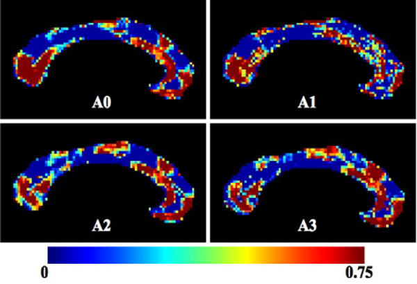
Heritability computed from the ICC. Red: more heritable regions h² = 0.75 - Blue: regions with no genetic influence h² = 0 - Top left: A0 no statistical information - Top right: A1 statistical information on the displacements - Bottom left: A2 statistical information on the deformation matrices - Bottom right: A3 both

4.2. Distance

Table 1 shows the ICC and its significance for each distance and all the algorithms (see 3.3) in the MZ group. As the corpus callosum is under genetic control, we estimate the robustness of our algorithm by comparing the ICC and p-value. The higher the ICC, the lower the p-value and the more identical the structures; registration errors tend to deplete the correlation between identical twins. The more significant statistics were found for algorithm 1 with d₁ and algorithm 0 with d₂. In Figure 2, we show the corresponding distances for the two algorithms previously mentioned. Each integer on the x-axis represents one MZ twin. The filled blue circles indicate the distance to that individuals twin sibling and the other colored circles the distance to the rest of the MZ population. In most cases, members of a twin pair were less distant from each than they were from the other subjects, suggesting the face validity of these metrics and the registrations from which they are derived.

Table 1.

Intraclass Correlation and its significance (p-value) computed for the two distances for each algorithm

		d1	d2
A0	ICC p-value	0.71 0.002	0.64 0.005
A1	ICC p-value	1 0	0.50 0.013
A2	ICC p-value	0.65 0.003	0.37 0.45
A3	ICC p-value	0.63 0.004	0.41 0.029

Fig. 2.

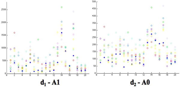
distance: left algorithm with dissipation with measure d1 right: algorithm without any stats with measure d2

5. CONCLUSION

In this paper, we introduced different algorithms using the Lagrangian framework, which differed in the type of statistical information incorporated in the regularization process. We chose to compare the power and robustness of these methods through the study of the corpus callosum, a heritable structure of the brain. Even though heritability maps give similar pattern, we noticed that including 1^rst order statistics (A2 and A3) in the deformation gave more powerful results (higher effect sizes). However, when we measured the robustness of the algorithms, the best results were given by the two other algorithms, that include no or 0^th order statistics, suggesting that they may provide more accurate registration. Including statistics on the displacement or the deformation gives promising results for improving power and robustness of registration for tensor-based morphometry. However, an implementation of these methods in 3D will help us determine more precisely the advantage of these statistical constraints on the registration process.

References

- 1.Arsigny, et al. Mag Res Med. 2006;56:411–421. doi: 10.1002/mrm.20965. [DOI] [PubMed] [Google Scholar]
- 2.Bajcsy, et al. Comp Vis Graph Image Process. 1989;46:1–21. [Google Scholar]
- 3.Bro-Nielsen, et al. VBC, Germany. 1996:272–276. [Google Scholar]
- 4.Brun, et al. ISBI, France. 2008 [Google Scholar]
- 5.Cachier, et al. MICCAI. PA, USA: 2000. pp. 472–481. [Google Scholar]
- 6.Cootes, et al. CVIU. 1995;61(1):38–59. [Google Scholar]
- 7.Chiang, et al. NeuroImage. 2007;34:44–60. doi: 10.1016/j.neuroimage.2006.08.030. [DOI] [PMC free article] [PubMed] [Google Scholar]
- 8.Christensen, et al. IEEE TIP. 1996;5:1435–1447. doi: 10.1109/83.536892. [DOI] [PubMed] [Google Scholar]
- 9.Hernandez, et al. MFCA, MICCAI. NY, USA: 2008. [Google Scholar]
- 10.Jenkinson NeuroImage. 2002;17:825–841. doi: 10.1016/s1053-8119(02)91132-8. [DOI] [PubMed] [Google Scholar]
- 11.Gee Pattern Recognition. 1999 [Google Scholar]
- 12.Gramkow . Master’s thesis. Denmark: 1996. [Google Scholar]
- 13.Grenander, et al. Quart of App Maths. 1998;56:617–694. [Google Scholar]
- 14.Hofer, et al. NeuroImage. 2006;32(3):989–994. doi: 10.1016/j.neuroimage.2006.05.044. [DOI] [PubMed] [Google Scholar]
- 15.Hulshoff Pol, Neurosci J. 2006;26:10235–42. [Google Scholar]
- 16.Leporé, et al. IEEE TMI. 2008;27(1):129–141. doi: 10.1109/TMI.2007.906091. [DOI] [PMC free article] [PubMed] [Google Scholar]
- 17.Leporé, et al. ISBI. Paris, France: 2008. [Google Scholar]
- 18.Miller NeuroImage. 2004;23(1):19–33. [Google Scholar]
- 19.Nichols, et al. HBM. 2002;15(1):1–25. doi: 10.1002/hbm.1058. [DOI] [PMC free article] [PubMed] [Google Scholar]
- 20.Pennec, et al. MICCAI. CA, USA: 2005. [Google Scholar]
- 21.Shattuck Med Image Anal. 2002;6:129–142. doi: 10.1016/s1361-8415(02)00054-3. [DOI] [PubMed] [Google Scholar]
- 22.Vercauteren, et al. IPMI. The Netherlands: 2007. [Google Scholar]