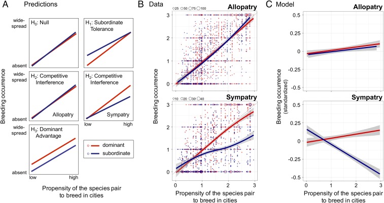
Fig. 2.
Predictions and test of hypotheses. (A) Predictions. Three alternative hypotheses and the null predict distinct patterns of breeding occurrence of birds in urban habitats. Lines show predicted patterns for dominant (red) and subordinate (blue) species. For H2, we distinguished between cities that occurred within (sympatry) or outside of (allopatry) areas of range overlap. (B) Data. In allopatry, breeding occurrence values of dominant and subordinate congeners were similar; in sympatry, dominant species were more widespread than subordinate congeners when species pairs had a high propensity to breed in cities. Each point in the figures represents the breeding occurrence of one species in one city (allopatry, n = 3,425; sympatry, n = 2,193); point size reflects the number of overlapping points (see legend at Top Left of graphs). Solid lines (red, dominants; blue, subordinates) are loess splines (span = 1.5) with 95% confidence limits shown in gray. Breeding occurrence values are means for each species in each city (averaged across observers, weighted by observer ability), and range from 0 (absent from urban habitats) to 3 (widespread breeder in urban habitats). Propensity to breed in cities was calculated for each paired dominant and subordinate species as the maximum breeding occurrence within a species pair for each city, averaged across all focal cities that overlapped their breeding ranges (one value per species pair; same value for sympatry and allopatry). (C) Model results. In allopatry, breeding occurrence values of dominant and subordinate congeners did not differ [Bayesian generalized linear mixed model (MCMCglmm), difference in slopes, PMCMC = 0.80]. In sympatry, dominant species were more widespread than subordinate congeners when species pairs had a high propensity to breed in cities (MCMCglmm, difference in slopes, PMCMC < 0.0001). Solid lines (red, dominants; blue, subordinates) are model-predicted values with 95% confidence limits in gray. Slopes in C are flattened relative to slopes in B because statistical models in C incorporated standardized breeding occurrence values (y axes) = [breeding occurrence value − mean(breeding occurrence for the species pair)]/[2 × SD(breeding occurrence for the species pair)]. See B for definition of propensity to breed in cities (x axis).

