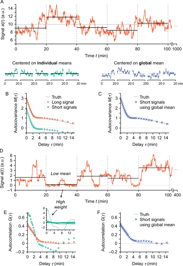
Fig. 2.

Biases due to the finiteness of time traces. (A) Shown is a portion of a signal used to illustrate the effect of inaccurate mean estimation. This 1000-min-long signal is partitioned into a set of 20-min-long signals. The true mean of the signal (ie, calculated on the long trace) is shown in gray and the inaccurate means of individual short traces are shown in black. (B) The autocovariance M(τ) of the entire signal shown in (A) is close to the expected curve (red circles vs gray curve). When averaging the autocovariances computed on each one of the 20-min-long traces, the resulting autocovariance deviates from the expected curve by a constant offset (green circles). (C) Performing the same calculation using a global estimation of the mean of the signals (ie, once over all the short signals) resolves the issue. (D) Another long signal is shown and partitioned into small sections to illustrate another artifact that may arise when averaging correlation functions G(τ). (E) The average (green circles) of the autocorrelation functions obtained on the 20-min-long sections of the signal shown in (D) deviates from the expected curve. This is due to an inaccurate weighting of the individual curves that occurs when averaging autocorrelation functions G(τ). As illustrated by the inset, the section that has a very low mean in (D) dominates the average. (F) As in (C), estimating the mean globally over all the signals solves the weighting problem. Both examples shown are simulated signals (A: Gaussian noise shaped in the Fourier domain, D: Monte Carlo simulation of transcription with Poisson initiation, distributed transcript dwell time and additive Gaussian noise). The “truth” curves in gray in (B), (C), (E), and (F) are the theoretical curves for both simulated situations.