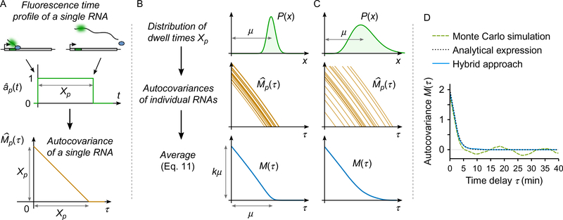
Fig. 5.

Principle of correlation function modeling. Although illustrated on a simplified single-color situation, the principle for modeling correlation functions presented here is general and holds for more complex descriptions. (A) Considering that the fluorescence time profile ${\widehat{a}}_p(t)$ recorded at the TS for a single nascent RNA is a rectangular function (rising when the MS2 cassette is transcribed and dropping when the RNA is release), then the covariance function ${\widehat{M}}_p(t)$ of this time profile is a triangle function. (B and C) When transcription initiation is considered homogeneous over time, the covariance function M(τ) can be understood as the average between individual correlation functions of single RNAs (Eq. 11). On the example of (A), if the dwell time X_p of individual RNAs is distributed, then the shape of M(τ) reveals information about initiation rate and dwell time distribution (mean, variability, etc.). (D) Several methods can be used to predict correlation functions from a given mechanistic scenario. As an alternative to a full Monte Carlo simulation approach, giving rather noisy results, and to analytical expressions, sometime difficult to derive, the hybrid approach described in Section 3.1.3 is both simple and precise. In this example, the hybrid method was performed over 100 single-RNA time profiles, and the simulation was performed over a signal that comprises 500 RNAs. The total computation time was similar in both cases. The analytical expression used is Eq. (12).