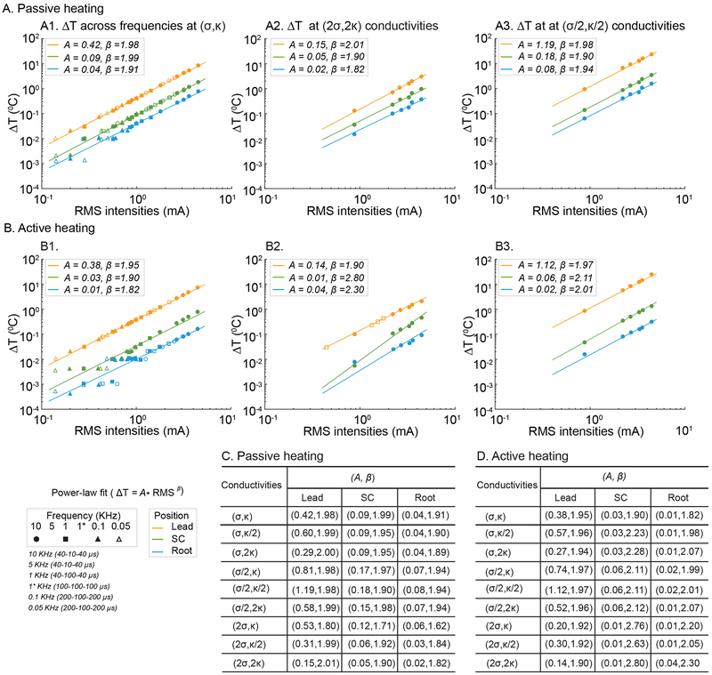
Fig 4: Power law-fit description of temperature increase with stimulation RMS in SCS model.
Temperature changes (ΔT) at three locations (Lead, orange; Spinal Cord, green; and Root, light-blue) as a function of stimulation RMS, across passive or active tissue model with varied fat electrical and thermal conductivity, were predicted by the FEM SCS model (data points). For each tissue model and compartment, we determined a best power-law fit (see Methods), which is a line with proportionality constant A and slope β (lines) on a log-RMS verse log-Temperature plot. Data plots include standard passive (A1), standard active (B1) tissue models, high thermal and electrical fat conductivity (2σ, 2κ) passive (A2) and active (B2) models, and low thermal and electrical fat conductivity (σ/2, κ/2) passive (A3) and active (B3). A and β across all 9 permutations of fat electrical (σ) and thermal (κ) conductivity are summarized for passive (C) and active (D) cases. RMS values plotted in A1 and A2 span stimulations frequencies of 0.05, 0.1, 1 (with low or high duty cycle), 5, and 10 KHz (waveforms indicated in legend and as used in Table 1). RMS values in A2, B2, A3 and B3 span 1, 5, and 10 KHz. A β > 1 indicates super-linear dependence of temperature rise on stimulation RMS; when β = 2 temperature increases with the square of RMS.

