Figure 1.

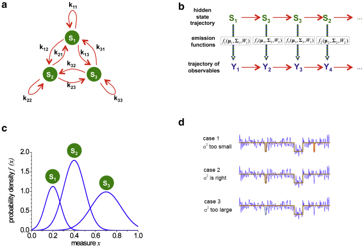
Principles of a hidden Markov model (HMM). (a) A scheme of a Markov model with three states (S1, S2, and S3) and their corresponding transition probabilities k_ij is shown. (b) A possible realization of a Markov chain is shown. For a series of states, the model emits an observable x_i based upon the actual state S_i and the probability density function f_i. This yields a trajectory of observables. In an HMM, the states themselves are not directly determinable because of noise and are hence hidden. The HMM analysis finds the parameters of the emission functions that best describe the data. From the given parameters, the Viterbi path is determined, which gives the most likely trajectory of hidden states that describes the observed data. (c) Three Gaussian emission functions with different means, variances, and occurrences are shown (μ_q = {0.2, 0.4, 0.7}, σ_q = {0.05, 0.1, 0.2}, W_q = {0.20, 0.45, 0.35}). (d) The influence of the variance on the state assignments extracted during an HMM analysis of an spFRET trace is depicted. When the variance is too small, the HMM introduces too many transitions, which yields a reduction in the duration of the individual states (case 1). When the variance is too large, state transitions are missed, which yields exaggerated state durations (case 3). When the variance models the broadness of a state correctly, the state durations are consistent with the transition probabilities (case 2). To see this figure in color, go online.