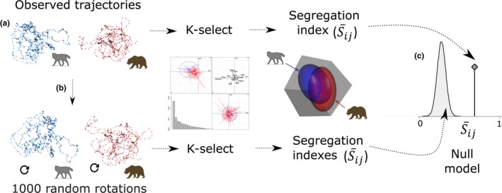
Figure 4.

Flowchart illustrating the procedure to analyze gray wolf and brown bear habitat selection and segregation in central Sweden. (a) Observed trajectories from each individual wolf and bear were used to quantify habitat selection with the K‐select (See Section 2.6). The four plots illustrate results obtained with the K‐select (Supporting Information Figures S3 and S4) which we used to calculate a segregation index (${\overline{S}}_{\mathit{ij}}$ = 0–100%) in terms of habitat selected by wolves and bears. This segregation index was calculated over all axes of the K‐select (i.e. weighted by the respective eigenvalues obtained on each axis). The 3D plot illustrates the habitat niche (ellipses) of wolves (blue) and bears (red) on only three different axes for illustrative purposes (${\overline{S}}_{\mathit{ij}}$ was actually performed on 18 different axes identified by the K‐select). The area of overlap between the two ellipses illustrates the area of overlap between wolves and bears, whereas the area outside represents habitat segregation. (b) To create random use of the habitat by both species, we randomly rotated the complete trajectory from each individual around its centroid 1,000 times. The same procedure described in (a) was used for each of the 1,000 simulated datasets. (c) The 1,000 segregation indexes were used to create the null model (density distribution curve: null hypothesis), the random distribution of the segregation index under random habitat used by both species. If the observed segregation index (vertical line, at the left of the density distribution curve) was ≥95% of the simulated segregation indexes, we rejected our null hypothesis and accepted our alternative hypothesis that segregation between both species was higher than expected by chance