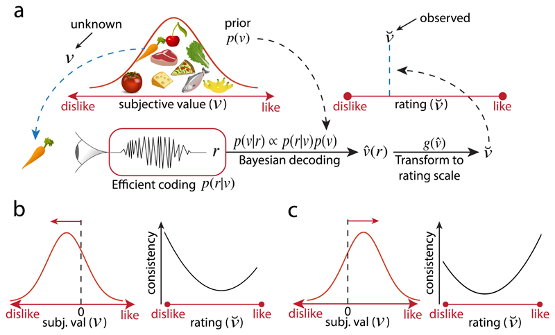
Figure 1. Simplified schema of the value inference model.
a) Observers infer the true value v of a food item by Bayesian inference constrained by efficient coding. The perceived food item with value value v elicits an internal response r. The corresponding likelihood function p(r|v) is constrained by the prior belief p(v) via efficient coding. In this example, the prior p(v) matches the distribution of subjective values v of supermarket products. The prior is combined with the likelihood to generate a posterior distribution p(v|r) via Bayes rule, to generate a subjective value estimate This estimate is subsequently mapped to the bounded rating scale imposed by the experimenter, resulting in an observed rating Crucially, unlike for experiments of perception, the experimenter has no access to the “true” stimulus value v that the participant uses to generate a rating. b,c) Choice consistency predictions as a function of the rating scale position (right plots in each panel) for two different priors (depicted on left of each panel). Prior distributions with higher density over low subjective values lead to higher choice consistency for low-valued goods (panel b); on the other hand, prior distributions with higher density over high subjective values lead to higher choice consistency for higher valued goods (panel c).

