Figure 7. Effects of D‐Aspartate treatment on corpus callosum demyelination.

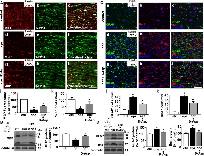
• A
  Representative confocal double immunofluorescence images displaying MBP (red) and NF200 (green) distribution and their coexpression (white) in the middle corpus callosum of septostriatal sections of control mice (a–c), and of mice fed with cuprizone for 5 weeks in the absence (d–f) or in the presence of D‐Asp (g–i). Scale bars in (a–i): 20 μm. (j), Densitometric analysis of MBP immunofluorescence signal and (k) quantification of MBP‐NF200 colocalized points in the middle corpus callosum of septostriatal sections from control mice, and from mice fed with cuprizone for 5 weeks in the absence or in the presence of D‐Asp.
• B
  Western blot and densitometric analysis of MBP levels in corpus callosum lysates from control and cuprizone‐treated mice for 5 weeks in the absence or in the presence of D‐Asp, respectively. Data were normalized on the basis of α‐tubulin and expressed as percentage of controls.
• C
  Representative confocal double immunofluorescence images displaying GFAP (green) and Iba1 (red) distribution in the middle corpus callosum of septostriatal sections of control mice (a–c) and of mice fed with cuprizone for 5 weeks in the absence (d–f) or in the presence of D‐Asp (g–i). Scale bars in (a–i): 50 μm. (j, k) Quantification of GFAP⁺ and Iba1⁺ cells in the middle corpus callosum of septostriatal sections of control mice and of mice fed with cuprizone for 5 weeks in the absence or in the presence of D‐Asp. Data were normalized to the total cell number (Hoechst signal) and expressed as percentage of controls.
• D
  Western blot (left panel) and densitometric analyses (middle and right panels) of GFAP and Iba1 protein levels in corpus callosum lysates obtained from control or cuprizone‐treated mice for 5 weeks in the absence or in the presence of D‐Asp.

Data information: The values represent the means ± SEM. Level of significance was determined by using in: (A, j) one‐way ANOVA P < 0.0001 followed by Bonferroni post hoc test, *P < 0.05 versus control, ^˄ P < 0.05 versus cpz (n = 4 mice for each group); (A, k) one‐way ANOVA P = 0.0162 followed by Newman–Keuls post hoc test, *P < 0.05 versus control, ^˄ P < 0.05 versus cpz (n = 4 mice for each group); (B) one‐way ANOVA P < 0.0001 followed by Bonferroni post hoc test, *P < 0.05 versus control, ^˄ P < 0.05 versus cpz (n = 3 mice for each group); (C, j, k) one‐way ANOVA P < 0.0001 followed by Bonferroni post hoc test, *P < 0.05 versus control, ^˄ P < 0.05 versus cpz (n = 4 mice for each group); (D) middle panel, one‐way ANOVA P = 0.0146 followed by Bonferroni post hoc test, *P < 0.05 versus control, ^˄ P < 0.05 versus cpz (n = 3 mice for each group); (D) right panel, one‐way ANOVA P = 0.0026 followed by Bonferroni post hoc test, *P < 0.05 versus control, ^˄ P < 0.05 versus cpz (n = 3 mice for each group). See the exact P‐values from comparisons tests in Appendix Table S7.Source data are available online for this figure.