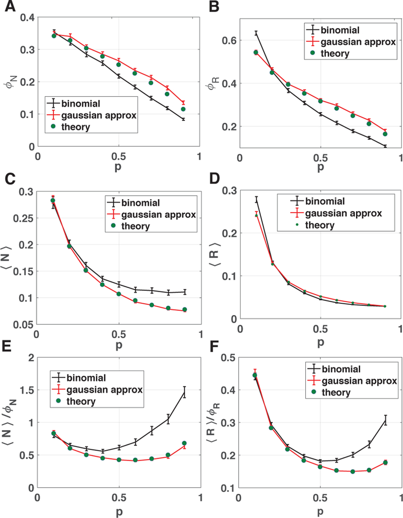
FIG. 2. Comparison of numerical simulations with theory.

Ecosystems were simulated with the consumption coefficients c_iα = 0, 1 drawn from a Bernoulli distribution with probability p (black lines) or a Gaussian distribution with same mean and variance as the binomial distribution (red line). Here S = M = 30, K = 1, σ_k = 1, m = 1, σ_m = .1, and 250 trials were used in these simulations: the error bars denote ±2 standard deviations. The K_a and m_i were drawn iid from a gamma distribution in the binomial plot to ensure nonnegativity of the parameters, and a Gaussian distribution in the Gaussian approximation plot. The numerical results were compared to theoretical predictions from the self-consistent cavity equations for ecologically stable steady-states (green circles). (A) Fraction of species that survive ϕ_N , (B) fraction of resources that are not depleted ϕ_R, (C) average abundance of all species 〈N〉, (D) average abundance of all resources 〈R〉 as a function of the probability p. (E) Mean-abundance of surviving species 〈N〉/ϕN and (F) mean-abundance of surviving resources 〈R〉/_R.