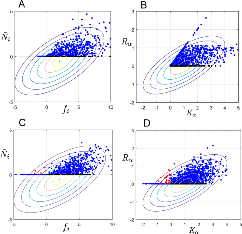
FIG. 4. Predicting the effective fttness and effective carrying capacity.

(A) Steady-state abundance ${\overline{N}}_i$ versus the fitness $f_i={\sum }_{\alpha }{c}_{i\alpha }\max \left\{K_{\alpha },0\right\}-m_i$ for each species i . Fitness is defined as the initial growth rate of species i in the environment in the absence of all other species. Points colored black are species with positive fitness that go extinct in the community $\left(f_i>0,{\overline{N}}_i=0\right)$. (B) Comparison of the steady state resource levels ${\overline{R}}_{\alpha }$ with their capacity K_α. The filled circles are generated from simulations with M = S = 30 resources and species, the data is generated from 50 separate trials. Parameters for simulations as in Figure 2 with p = and σm/m = 0.1. Black points indicate resources which have a positive capacity but go extinct in the community. The difference between plots for (A,B) and (C,D) is that in the former K_α and m_i are always positive because they are drawn from a gamma distribution and Bernoulli distribution respectively. In (C,D), each of these parameters is drawn from a Gaussian distribution with the same mean and variance as in (A,B). This means that a small fraction of the K_α, m_i, and c_iα are negative. Negative c_iα corresponds to production of resource α by species i at a fitness cost to itself (i.e. public good production). In (C,D), red points indicate species with negative fitness that can stably exist in the community $\left(f_i<0,\text{}{\overline{N}}_i>0\right)$ or resources with negative K_α that are produced by the ecosystem. Contours show theoretical predictions of our CM for correlation between${\overline{N}}_i$ and f_i as well as ${\overline{R}}_{\alpha }$ and K_α (see Appendix E for details). Each contour represents half a standard deviation of our theory.