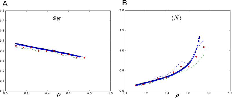
FIG. 5. Comparing CRM theory vs simulation - another setting.

All parameters defining the species were drawn from a Gaussian distribution as in main text but with σ_m = 1 (a larger maintenance cost variance). Interestingly, we see a difierent behavior than in Fig 2 in that the average abundance 〈N〉 of all species is increasing with increasing niche overlap. Also, the number of surviving species is reduced by high niche overlap as it is in Fig 2, which makes sense since when species are very similar they will compete more directly for the same resources. The parameters used are: σ_m = 1; m = 1; σ_k = 1; K = 1, and simulations were run assuming an equal number of species and resources S = M = 30 (γ = 1). Additionally, μ_c = 1 was fixed and σ_c varied (note that the niche overlap ρ is determined by these two variables). The theoretical predictions from the cavity solution (blue), match well with the numerical solutions (red) for the CRM model averaged over 100 trials with and plotted with ±2 standard deviation error bars (dashed lines).