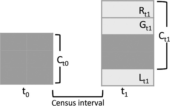
Figure 1.

Schematic model representing the different components of forest demography. The box on the left represents an inventory plot of a forest community at the first census (C _t0), while the box on the right shows the community at the second census (C _t1). At C _t1 recruits (R), that is those trees that attained 10 cm of diameter within the census interval, will now be part of the community analysed. Other trees will have died thus leaving the community, here called losses (L). Those trees from C _t0 that survive through the census interval are expected to grow (G). Thus, the basal area of the whole community at t ₁ is C _t1 = C _t0 + G _t1 + R _t1 − L _t1 and the net flux between t ₀ and t ₁ = G _t1 + R _t1 − L _t1. Here we investigate the trends in the characteristics and identity of genera within these components of forest demography. This figure represents dynamics in basal area terms; similar logic can be applied for stem‐based analyses. Note that in this case we would not be interested in the growth of trees surviving from t ₀ to t ₁, and so the net flux would be represented as R _t1 − L _t1