. 2019 Jan 16;8:e39595. doi: 10.7554/eLife.39595

Figure 1. Outline and results of pooled ATAC-seq.

(A) Performing ATAC-seq in a pool of individuals selects DNA molecules with higher CA, thus enriching for more accessible alleles. In this example (ASW population), the G allele has a low pre-ATAC frequency but a high post-ATAC frequency, due to its increased CA. The ten population abbreviations refer to: CEU, Utah residents with North European ancestry; FIN, Finnish; TSI, Tuscan; IBS, Iberian; ASW, African-American from Southwest US; YRI, Yoruban; ESN, Esan; LWK, Luhya; GWD, Gambian; and CHB, Han Chinese. (B) The number of caQTLs (top), and the percent of all tested SNPs called as caQTLs (bottom). (C) Enrichment of caQTLs among dsQTLs (Degner et al., 2012), at a range of caQTL p-value cutoffs. (D) Quantitative effect sizes of caQTLs and dsQTLs are highly correlated (scales of each axis are not comparable, and do not affect the correlation coefficient).( E–F) The degree of allelic concordance between our caQTLs and: (E) dsQTLs (Degner et al., 2012). (F) bQTLs aggregated for five TFs (Tehranchi et al., 2016). Full results available in Figure 1—source data 1.

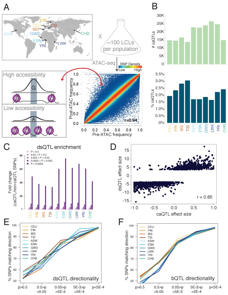
Figure 1—source data 1. Detailed results of analyses shown in the Figures.
Each tab has a separate summary: caQTL summary: Numbers of cell lines, reads, SNPs, and caQTLs Shared caQTL summary: Number of populations in which each shared caQTL reached p<0.005 Individual coefficients: The coefficients inferred from our regression approach for inferring contribution of each sample to each pool Numbers of QTLs: Total numbers of dsQTLs, bQTLs, and Hi-C GM12878 heterozygous SNPs used in our analyses Fig 1C-F: Numbers going into Figure 1C–F.
DOI: 10.7554/eLife.39595.008

Figure 1.

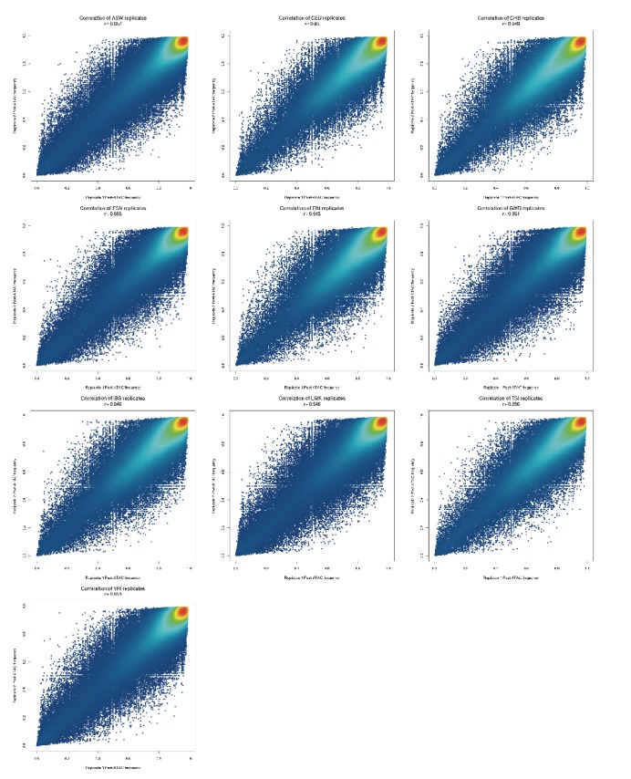
Figure 1—figure supplement 1. Comparison of post-ATAC reference allele frequencies between biological replicates of each population pool.

Figure 1—figure supplement 1.

All replicates have 0.94 < r < 0.96.
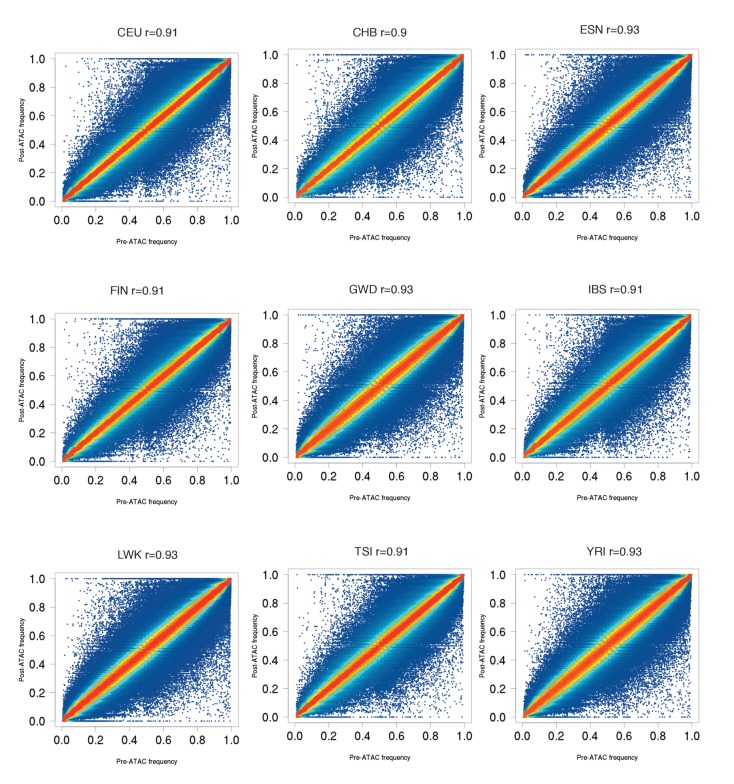
Figure 1—figure supplement 2. Pre-ATAC vs post-ATAC reference allele frequencies for nine populations, similar to ASW plot in Figure 1A.

Figure 1—figure supplement 2.

Most SNPs fall close to the diagonal, as expected if most SNPs are not caQTLs. All populations have 0.90 < r < 0.94.
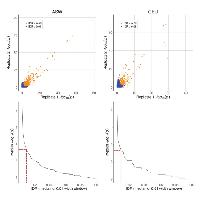
Figure 1—figure supplement 3. Top row: caQTL p-values for SNPs on chr one in ASW and CEU, shown separately for each biological replicate.

Figure 1—figure supplement 3.

Bottom row: median –log10(p-value) as a function of IDR, plotted using a moving window of IDR values (window width = 0.01). Dashed red lines indicate the p-value cutoff of 5 × 10⁻⁴, corresponding to IDR ≈ 0.01.
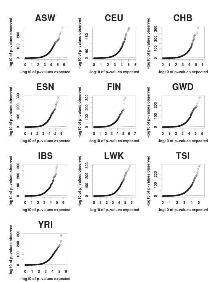
Figure 1—figure supplement 4. QQ plots of expected (under the null) vs observed caQTLs p-values.

Figure 1—figure supplement 4.

All populations show a similar excess of significant p-values.
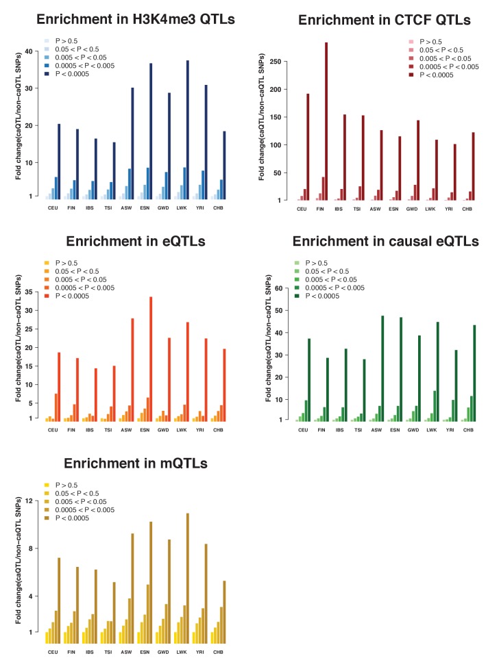
Figure 1—figure supplement 5. caQTLs enrichments among other molecular QTLs (Ding et al., 2014, Lappalainen et al. (2013), Waszak et al., 2015, Tewhey et al., 2016, Banovich et al., 2014).

Figure 1—figure supplement 5.