Diagnosis of mesothelioma with deep learning

Abstract

Malignant mesothelioma (MM) is a rare but aggressive cancer. The definitive diagnosis of MM is critical for effective treatment and has important medicolegal significance. However, the definitive diagnosis of MM is challenging due to its composite epithelial/mesenchymal pattern. The aim of the current study was to develop a deep learning method to automatically diagnose MM. A retrospective analysis of 324 participants with or without MM was performed. Significant features were selected using a genetic algorithm (GA) or a ReliefF algorithm performed in MATLAB software. Subsequently, the current study constructed and trained several models based on a backpropagation (BP) algorithm, extreme learning machine algorithm and stacked sparse autoencoder (SSAE) to diagnose MM. A confusion matrix, F-measure and a receiver operating characteristic (ROC) curve were used to evaluate the performance of each model. A total of 34 potential variables were analyzed, while the GA and ReliefF algorithms selected 19 and 5 effective features, respectively. The selected features were used as the inputs of the three models. SSAE and GA+SSAE demonstrated the highest performance in terms of classification accuracy, specificity, F-measure and the area under the ROC curve. Overall, the GA+SSAE model was the preferred model since it required a shorter CPU time and fewer variables. Therefore, the SSAE with GA feature selection was selected as the most accurate model for the diagnosis of MM. The deep learning methods developed based on the GA+SSAE model may assist physicians with the diagnosis of MM.

Introduction

Malignant mesothelioma (MM) is a rare but aggressive cancer (1). The prognosis of patients with MM is poor since the majority of patients are diagnosed at an advanced stage and MM is resistant to current treatment options, including chemotherapy, surgery, radiotherapy and immunotherapy (2). The estimated median overall survival for advanced MM is 1 year following diagnosis (3). MM has a strong association with exposure to asbestos, a mineral extensively used worldwide in the 1970-80s. Although the use of asbestos has been prohibited in the 21st century, the incidence rate of MM has continued to increase worldwide due to the long latency period of MM (2,4).

Diagnosis of MM primarily relies on histopathological examination supported by clinical and radiological evidence (5). The definitive diagnosis of MM is a crucial step prior to appropriate treatment and has important medicolegal significance due to diagnosis-related compensation issues (6). However, the definitive diagnosis of MM can be complex, particularly during early stages. This is due to significant variation between cases and the presence of traits that mimic other cancers (particularly adenocarcinoma) or benign/reactive processes (6). Furthermore, given the low frequency of MM, it is commonly misdiagnosed or not identified due to a lack of experienced pathologists (1,6).

In the last two decades, the use of diagnosis support systems (DSSs) has gradually increased (7–9). A DSS for MM may enable pathologists to rapidly examine medical data in considerable detail. More importantly, it may reduce the variability that occurs with different pathologists. Previous studies regarding computer-aided diagnosis of MM mainly focused on developing automatic image processing approaches, including methods that can automatically detect and quantitatively assess pleural thickening in thoracic computed tomography images (10–12). However, pleural thickening does not exclusively signify an asbestos-related disease (3), therefore previous methods possess limitations for identifying MM. To increase the accuracy of the DSS, it is necessary to effectively combine multi-feature data, including clinical, laboratory and radiological characteristics of MM. Er et al (7) collected multi-feature data to diagnose MM. The authors achieved 96.30% classification accuracy by using a probabilistic neural network (PNN). However, multi-feature data may not contribute equally to the identification of MM. Feature selection methods may be utilized to remove the redundant or irrelevant features from the original feature set (9); this may aid the diagnosis model to focus on the most discriminative features in order to achieve a higher accuracy and decrease the learning time.

Disease diagnosis is a major classification issue; therefore, the classifier is critical to the DSS. Previously, a number of machine leaning methods have been used as classifiers to assist the diagnosis of disease, including support vector machine (13,14), extreme learning machine (ELM) (15) and deep learning (DL; also termed Hierarchical Learning) (16,17). DL facilitates computational models, consisting of multiple processing layers, to learn representations of data with multiple levels of abstraction (18). DL is a family of computational methods, which includes the restricted Boltzmann machine (19), stacked autoencoder (20), deep belief networks (21) and convolutional neural networks (22). These algorithms markedly improve speech recognition, object detection and visual object recognition (16,23).

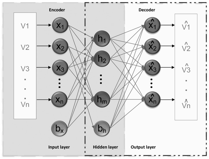
An autoencoder is a type of neural network including three layers: input layer, hidden layer, and output layer (20). Fig. 1 presents the architecture of a basic autoencoder with ‘encoder’ and ‘decoder’ networks. An extension of an autoencoder, the sparse autoencoder (SAE) introduces a spare constraint on the hidden layer (20). Its algorithm steps are as follows: The given dataset, X={x(1), x(2),…, x(i)… x(N)}, x(i) ∈R^M is mapped to the hidden layer with a nonlinear activation function:

Figure 1.

Architecture of a basic autoencoder. V (1,2…n), entire training data; X (1,2…n), set of training data; b_h, bias of hidden layer; b_x, bias of input layer; h (1,2…m), feature vector at hidden layer; xˆ, reconstruction of input x.

$$Z=f(W_{1}X+b_1)=\frac{1}{1+exp[-(W_{1}X+b_1)]}$$

Then, the resulting hidden representation Z is mapped back to a reconstructed vector h_w,b(x) in the input space.

$$h_{w,b}(x)=f(W_{2}Z+b_2)=\frac{1}{1+exp[-(W_{2}Z+b_2)]}$$

In the aforementioned formulas, X represents the feature expression of the original data, R represents real numbers; N represents the number of data samples and M represents the length of each data sample. W₁ represents the weight matrix and b₁ represents the bias of the encoder. f represents the encoder activation function. Subsequently, the parameter set, W₁, b₁, W₂, b₂, are optimized by minimizing error between the input and reconstructed data. The cost function of the SAE can be written as:

$$J(W,b)=\frac{1}{N}\sum _{i=1}^N\left(\frac{1}{2}{\Vert h_{w,b}(x(i))-x(i)\Vert }^2\right)+\frac{\lambda }{2}\sum _{l=1}^2\sum _{i=1}^{S_l}\sum _{j=1}^{S_{l+1}}{\left(W_{ji}^l\right)}^2+\beta \sum _{j=1}^{S_2}KL(\rho \Vert {\hat{\rho }}_j)$$

In this formula, N represents the number of data samples, h_w,b(x(i)) represents the output feature vector, x(i) represents the input feature vector, λ represents the weight decay parameter, S_l represents the number of neurons in layer l, β represents the weight of sparsity penalty term, W^l_ji represents the weight on the connection between neuron j in layer l+1 and neuron i in layer l, ρ represents the sparsity parameter defining the sparsity level and ρ_j represents the average activation of hidden neuron j. ^{$KL(\rho \Vert \hat{\rho }\mathrm{i})$} represents the Kullback-Leibler divergence between ^ρ and ^{$\hat{\rho }\mathrm{i}$}.

By minimizing J(W,b) the optimal parameters of W and b are updated in the process of coding. The parameters W and b in each iteration can be updated as:

$$W_{ji}^l=W_{ji}^l-\epsilon \frac{\partial }{\partial W_{ji}^l}J(W,b)\text{and}{b}^l=b^l-\epsilon \frac{\partial }{\partial b^l}J(W,b)$$

In these formulas, parameter ε represents the learning rate; l represents the l^th layer of the network; i and j denote the i^th and j^th neurons of two neighboring layers, respectively. J(W,b) represents the cost function of the SAE and ∂ represents seeking partial derivative.

Stacked sparse autoencoder (SSAE) is a newly developed DL algorithm and a feed-forward neural network consisting of multiple layers of basic autoencoder. SSAE has successfully been employed to identify visual features in computer vision (24,25), predict protein solvent accessibility and contact number (26), predict protein-protein interactions (27) and construct an electronic nose system (28). Similar to other DL algorithms, SSAE can efficiently use a deep or layered architecture to identify potential representations from original clinical features, therefore enhancing the classification accuracy (20).

However, the performance of classification algorithms may differ from one dataset to another (29). Different classification algorithms may be used to develop and compare several models, allowing the best solution to be selected based on the dataset (29). In the current study, the GA and ReliefF methods were used to select high discriminative features and three commonly used machine leaning algorithms, BP, ELM and SSAE were selected as the classification algorithms. The performance of these models was compared using evaluation metrics, including classification accuracy, specificity, F-measure and AUC. The model with the best performance may be considered as a classifier to be used when developing a DSS to diagnose MM.

Materials and methods

Data source

To facilitate comparisons with previous studies, the current study used a dataset obtained from the University of California (Irvine, CA, USA) machine learning database (7). The original dataset includes 324 participants. For each participant, 34 physiological variables were recorded, as presented in Table I.

Table I.

Variables for diagnosing malignant mesothelioma.

Variable	Value type
Age	Quantitative
Sex	Qualitative
City	Qualitative
Asbestos exposure	Qualitative
Type of malignant mesothelioma	Qualitative
Duration of asbestos exposure	Quantitative
Diagnosis method	Qualitative
Keep side	Qualitative
Cytology	Qualitative
Duration of symptoms	Quantitative
Dyspnoea	Qualitative
Ache on chest	Qualitative
Weakness	Qualitative
Smoker	Qualitative
Performance status	Qualitative
White blood cell count	Quantitative
Hemoglobin	Quantitative
Platelet count	Quantitative
Sedimentation rate	Quantitative
Blood lactose dehydrogenase	Quantitative
Alkaline phosphatase	Quantitative
Total protein	Quantitative
Albumin	Quantitative
Glucose	Quantitative
Pleural lactose dehydrogenase	Quantitative
Pleural protein	Quantitative
Pleural albumin	Quantitative
Pleural glucose	Quantitative
Mortality	Qualitative
Pleural effusion	Qualitative
Pleural thickness on tomography	Qualitative
Pleural pH	Qualitative
Cell count	Quantitative
C-reactive protein	Quantitative

Data preprocessing and feature selection

The original dataset was classified into two groups by experienced pathologists: 97 patients with MM and 227 healthy participants. For each participant, 34 variables were recorded and no data were missing. Multiplicity of the features may lead to over-training a model. Therefore, a frequently used preprocessing method is feature selection, in which irrelevant, weakly relevant or less discriminative features are removed. Feature selection can increase the accuracy of the resulting model (30,31). Previously, a variety of feature selection algorithms have been developed to perform feature selection (32,33). The current study used the GA (34) and the ReliefF algorithm (30) with MATLAB software (R2016b 9.1.0.441655); MathWorks, Natick, MA, USA). The parameters of GA were set as follows: Number of generations=100, population size=20, encoding length=34 and the crossover rate=2. While ReliefF methods were used to select high discriminative features, the parameters of ReliefF were set as follows: Number of iterations=323 and the number of close samples=95. The important features selected by GA and ReliefF were used as inputs to train the diagnosis models. For training these diagnosis models, the dataset was randomly divided into training (70%) and testing (30%) data.

Construction of the diagnosis models

Previous studies have demonstrated that the most effective model is not always easily identified. Therefore, testing various diagnosis models is required to select the most effective one. In the current study, a number of diagnosis models, including BP, ELM and SSAE, were developed using MATLAB software. Selected features were used as the inputs for these recognition models.

The algorithm principle for BP can be reviewed in a previous study (35). In the current study, the parameters of BP were set as follows: Size of hidden layers=50, transfer function of hidden layers=‘tansig’, transfer function of output layer=‘purelin’, training function=‘trainlm’, epoch =1,000, goal of training accuracy=0.1 and the learning rate=0.1. Other associated parameters were based on the default values of MATLAB.

In addition, an ELM algorithm was selected to build a pattern recognition model. ELM is a learning algorithm, which is developed on the basis of a single-hidden layer feed-forward neural network (15). ELM can achieve a faster learning speed and improved generalization capability compared with other pattern recognition models by distributing the input weights and hidden layer biases randomly and determining the output weights through a Moore-Penrose generalized inverse operation of the weight matrices in hidden layers (36). Further information regarding ELM can be reviewed in a previous study (37). In the current study, the number of hidden nodes was set to 30 and the sigmoidal function was adopted as the transfer function.

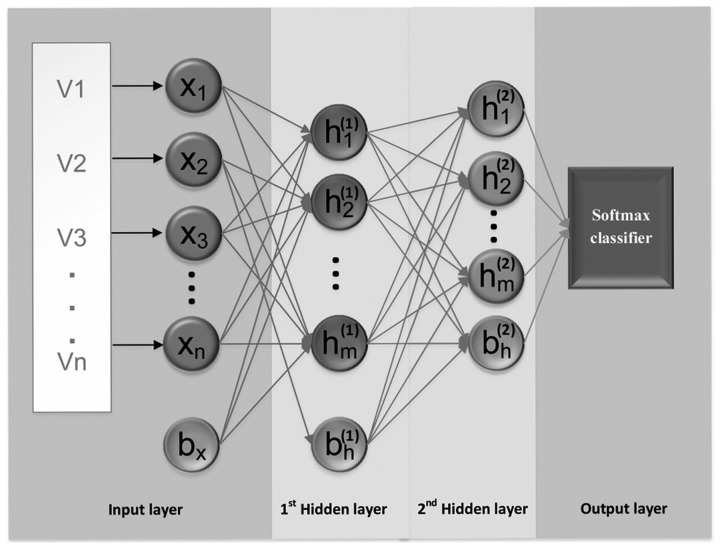
The SSAE is a feed-forward neural network consisting of multiple layers of basic autoencoder (28). To reduce the dimensions and extract high-level abstract features from the input without labels, two autoencoders were stacked to generate an SSAE in the current study. When using an SSAE, features calculated by the first autoencoder are used as the inputs for the second autoencoder's hidden layer, as presented in Fig. 2. When the expected error rate is achieved by the first autoencoder, the high-level abstract features are extracted by the second autoencoder (38,39). In the current study, a supervised model, the Softmax classifier (SMC), was connected to the end of the trained SSAE to identify the classification task. To train the SMC, the high-level abstract features extracted by the SSAE were used as the inputs for the softmax layer. Following training, the SMC was stacked with SSAE to establish a deep neural network (Fig. 2). Further information regarding the SMC can be reviewed in previous studies (38,40).

Figure 2.

Architecture of sparse autoencoder. V (1,2…n), entire training data; X (1,2…n), set of training data; b_h, bias of hidden layer; and b_x, bias of input layer; h^(l) (1,2…m), feature vector at layer l; h⁽²⁾ (1,2…m), feature vector at layer 2.

The parameters of the first autoencoder were set as follows: When using raw data as the input the size of the hidden representation=30, when using data generated by dimension reducing processing as the input the size of the hidden representation=20, weight regularization for loss function=0.001, sparsity regularization for loss function=4 and sparsity proportion=0.05. The parameters of the second autoencoder were set as follows: Size of the hidden representation=10, weight regularization for loss function=0.001, sparsity regularization for loss function=4 and sparsity proportion=10. In addition, the current study selected the linear transfer function.

Performance measure

In order to evaluate and select the most accurate diagnostic model, confusion matrixes were adopted to calculate the sensitivity, specificity, precision and accuracy of each diagnostic model. Occasionally, contradictions occurred between the sensitivity and precision, therefore the F-measure was used to weight and average the two values: F=(2 × precision × sensitivity)/(precision+sensitivity).

In addition, a receiver operating characteristic (ROC) curve and the area under the ROC curve (AUC) were used to evaluate the performance of the diagnostic models. ROC analysis evaluated the capacity of the diagnostic models to distinguish between MM and healthy participants. All calculations were based on standard equations published in previous studies (31,41). Furthermore, the central processing unit (CPU) time was recorded and compared between the SSAE and GA+SSAE diagnostic models to indicate the computational complexities of each model.

Results

Identifying variables that are important for MM diagnosis by feature selection

The original dataset contained 34 variables for each participant. GA and ReliefF were performed to select the most significant features for diagnosing MM. 19 relevant features were selected as the feature subset based on GA. However, only five relevant features with a weight value >0.10 were selected as the feature subset based on the ReliefF algorithm. The feature subset based on GA included: Age, gender, city, duration of asbestos exposure, diagnosis method, cytology, ache on chest, weakness, smoking habit, white blood cell level, hemoglobin level, blood lactose dehydrogenase level, albumin level, glucose level, pleural lactose dehydrogenase level, pleural protein level, pleural glucose level, cell count and pleural level of acidity.

Comparing the diagnostic models

The current study compared the performance of the diagnosis models using four evaluation measures, as illustrated in Figs. 3–6. Overall, SSAE and GA+SSAE demonstrated a higher performance compared with the other diagnosis models evaluated.

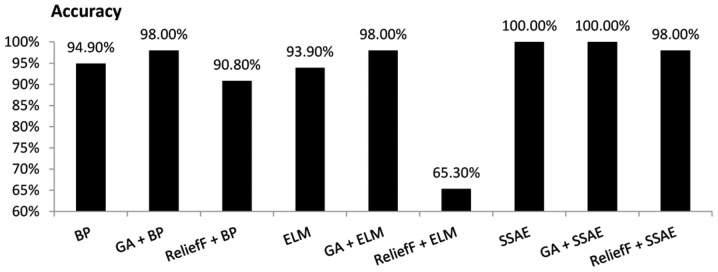
Figure 3.

Comparison of the accuracy achieved by various diagnostic models. BP, backpropagation; GA, genetic algorithm; ELM, extreme learning machine; SSAE, stacked sparse autoencoder.

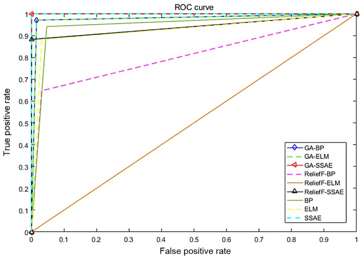
Figure 6.

ROC curves to assess the capacity of the diagnostic models to distinguish between patients with malignant mesothelioma and healthy participants. ROC, receiver operating characteristic; BP, backpropagation; GA, genetic algorithm; ELM, extreme learning machine; SSAE, stacked sparse autoencoder.

When all 34 variables of the original data set were used to diagnosis MM, the SSAE model demonstrated the highest accuracy (100.00%), while other models demonstrated an accuracy <95%. When the 19 variables selected by GA were used as the input variables, both the GA+BP and GA+ELM models achieved an accuracy of 98.00%. However, GA+SSAE demonstrated the highest accuracy (100.00%). When the five variables selected by the ReliefF algorithm were used as the input variables, the accuracy of the ReliefF+SSAE model decreased to 98.00%, while the other models demonstrated accuracies <92% (Fig. 3).

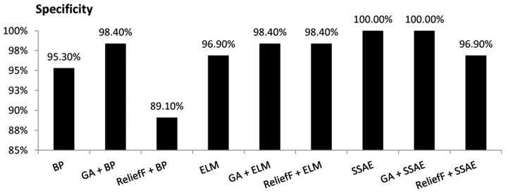
The SSAE model demonstrated a specificity of 100.00% when all 34 variables of the original data set were used as the input variables. Similarly, when the 19 variables selected by GA were used as the inputs, the GA+SSAE model demonstrated a specificity of 100.00%. By contrast, the ReliefF+BP model achieved the lowest specificity of 89.10% (Fig. 4).

Figure 4.

Comparison of the specificity achieved by various diagnostic models. BP, backpropagation; GA, genetic algorithm; ELM, extreme learning machine; SSAE, stacked sparse autoencoder.

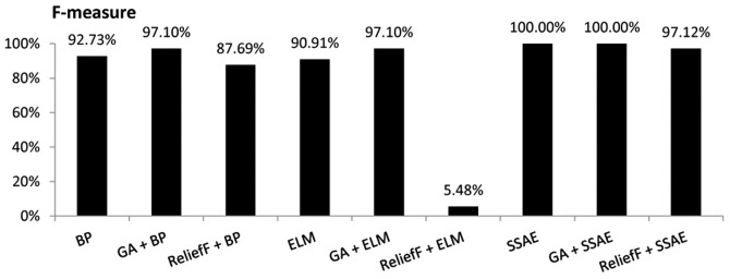
When all 34 variables of the original data set were used as the inputs, the SSAE model demonstrated the highest F-measure value (100.00%), while ELM achieved the lowest F-measure value (90.91%). When the 19 variables selected by GA were used as the input variables, both GA+BP and GA+ELM models demonstrated an F-measure value of 97.10%. With the same input variables, the GA+SSAE model achieved the highest F-measure value (100.00%). However, when the five variables selected by the ReliefF algorithm were used as the input variables, the F-measure value of the ReliefF+ELM model decreased markedly to 5.48%, while the F-measure value of the ReliefF+SSAE model was 97.12% (Fig. 5).

Figure 5.

Comparison of the F-measure for various diagnostic models. BP, backpropagation; GA, genetic algorithm; ELM, extreme learning machine; SSAE, stacked sparse autoencoder.

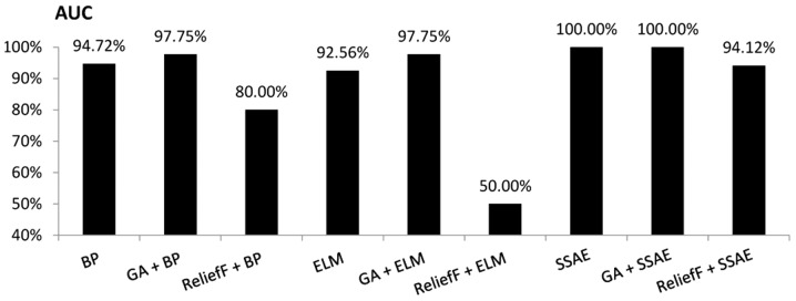
An evaluation was performed to compare the discriminatory power of the BP, ELM and SSAE models, with or without feature selection, as illustrated in Figs. 6 and 7. An ROC curve and the AUC were used to indicate the effectiveness of a diagnostic model to discriminate between patients with MM and healthy participants. The current study revealed that the SSAE and GA+SSAE models demonstrated the highest diagnostic power compared with the other models, as presented in Fig. 7.

Figure 7.

Comparison of the area under the receiver operating characteristic curves for various diagnostic models. AUC, area under the curve; BP, backpropagation; GA, genetic algorithm; ELM, extreme learning machine; SSAE, stacked sparse autoencoder.

Performing feature selection does not exclusively improve the performance of diagnostic models

As demonstrated in Figs. 3–7, performing GA markedly enhanced the classification performance of BP. Compared with BP alone, GA+BP achieved a higher accuracy (98.00 vs. 94.40%), specificity (98.4 vs. 95.30%), F-measure (97.10 vs. 92.73%) and AUC (97.75 vs. 94.72%). Whereas, compared with BP alone, performing a ReliefF algorithm generated a lower accuracy (90.80 vs. 94.90%), specificity (89.10 vs. 95.30%), F-measure (87.69 vs. 92.73%) and AUC (80 vs. 94.72%).

As demonstrated in Fig. 4, performing GA or ReliefF prior to training the ELM classifiers markedly improved the specificity. Compared with ELM alone, the GA+ELM model revealed a higher accuracy (98.00%), specificity (98.40%), F-measure (97.10%) and AUC value (97.75%). However, comparison of the accuracy, F-measure and AUC demonstrated that performing the ReliefF algorithm reduced the performance of the ELM model on the same dataset.

The performance of SSAE in diagnosing MM was compared with that of the GA+SSAE and ReliefF+SSAE models. In comparison with SSAE without feature selection, performing the ReliefF algorithm achieved a worse performance. However, both SSAE and SSAE+GA achieved an accuracy, specificity, F-measure and AUC of 100%. The average CPU time of the SSAE diagnostic model following GA feature selection was compared with the average CPU time of the baseline SSAE diagnostic model without feature selection. Each model was performed ten times. the mean CPU time of SSAE was 33.2 sec. However, following GA feature selection, the mean CPU time of SSAE decreased to 28.8 sec.

Discussion

The definitive diagnosis of MM is significant at both the individual and public health level, and has important medicolegal significance due to diagnosis-related compensation issues (6). However, the definitive diagnosis of MM is complicated due to its composite epithelial/mesenchymal pattern and its low occurrence frequency (6). To improve the diagnosis of MM at an early stage, the current study designed and implemented a diagnostic model based on SSAE algorithms.

To the best of our knowledge, no previous studies have developed MM diagnostic models using SSAE algorithms. However, previous studies have successfully applied SSAE in processing diagnosis information (38,40,42). A number of previous studies have compared the performance of different statistical and machine learning techniques in the field of medical diagnosis; the results revealed that the performance of SSAE is higher than several other similar techniques (42,43), a finding that is consistent with the current study.

However, the performance and precision of a classification algorithm may vary depending on the dataset (44). For a specific dataset, it is difficult to identify which classification algorithm has the highest performance without performing a comparison. In addition, feature selection methods exhibit a marked influence on the performance of a classification algorithm; a feature subset that improves the performance of one classification algorithm may not improve the performance of a different classification algorithm. To generate a diagnostic model for MM and evaluate its performance, three different algorithms with or without feature selection were applied on the same training dataset and their performances were compared in the current study.

The results indicated that the SSAE and GA+SSAE models exhibited the highest overall performance; the accuracy, specificity, F-measure and AUC for both models were 100%. However, following feature selection with GA a decrease was identified in the CPU time for training the SSAE diagnostic model compared with the baseline SSAE diagnostic model without GA. Furthermore, the GA+SSAE model required fewer variables to achieve the same performance as SSAE. The ReliefF+ELM diagnosis model exhibited the worst performance on the dataset used in the current study, with an accuracy, F-measure and AUC of 65.30, 5.48 and 50.00%, respectively. In addition, performing feature selection did not exclusively produce an improved performance. The accuracy of the ReliefF+ELM model was 65.3%, while the accuracy of ELM without feature selection was 93%. Similarly, the ReliefF algorithm reduced the performance of the SSAE model.

The results from the current study were compared with a previous study that used the same training dataset (7). The previous study compared the performance of three classification methods and identified that the classification accuracies were 96.30, 94.41 and 91.14% for PNN, multilayer neural network and learning vector quantization structures, respectively. The highest classification accuracy was obtained using a PNN (with 3 fully connected layers, response surface method) structure (96.30%) (7,45). In comparison, the SSAE and GA+SSAE methods achieved a classification accuracy of 100% on the same training dataset, in the current study.

The current study demonstrates the effectiveness of DL in the diagnosis of cancer. A pathologist's clinical impression and diagnosis of MM is based on contextual factors, whereas a GA+SSAE model has the ability to diagnose MM with high accuracy and may augment clinical decision-making. Furthermore, this fast and scalable method may be applied to other clinical datasets for the diagnosis or prediction of other cancer types.

In conclusion, the current study has aimed to improve the diagnosis of MM by evaluating three deep learning algorithms, using a dataset containing 97 patients with MM and 227 healthy participants. To avoid over-training and improve the classification accuracy of a diagnosis model, ReliefF and GA feature selection algorithms were implemented to remove the irrelevant or weakly relevant features. The current study identified that the GA+SSAE algorithm exhibited the highest performance in all evaluation criteria and required the smallest number of variables. The GA+SSAE algorithm-based DSS may contribute to the definitive diagnosis of MM. Consequently, the current study may assist pathologists with the diagnosis of MM by providing a system that can achieve optimal diagnostic performance. In addition, it may facilitate the screening of high-risk individuals in regions where asbestos exposure is common.

Funding

The current study was supported by the Foundation and Frontier Research Project of Chongqing (grant no. cstc2016jcyjA0526), the Science and Technology Research Project of Chongqing Municipal Education Committee (grant no. KJ1600519), the Technology Innovation Project of Social Undertakings and Livelihood Security of Chongqing (grant no. cstc2017shmsA30016) and the Postgraduate Science and Technology Innovation Project of Chongqing (grant nos. CYS17215 and CYS17203).

Availability of data and materials

The datasets analyzed during the current study are available in the University of California (Irvine, CA, USA) machine learning database, https://archive.ics.uci.edu/ml/datasets/Mesothelioma %C3%A2%E2%82%AC%E2%84%A2s+disease+data+set+.

Authors' contributions

ZY and XH contributed to the conception of the study. XH contributed to analysis and manuscript preparation. ZY and XH performed the data analyses and wrote the manuscript. ZY and XH helped perform the analysis with constructive discussions.

Ethics approval and consent to participate

The current study used a dataset obtained from a public database. The data submitters have gain informed consent for publication of the dataset from participants at the point of recruitment to the trial.

Patient consent for publication

Not applicable.

Competing interests

The authors declare that they have no competing interests.

References

- 1.Remon J, Lianes P, Martinez S, Velasco M, Querol R, Zanui M. Malignant mesothelioma: New insights into a rare disease. Cancer Treat Rev. 2013;39:584–591. doi: 10.1016/j.ctrv.2012.12.005. [DOI] [PubMed] [Google Scholar]
- 2.Remon J, Reguart N, Corral J, Lianes P. Malignant pleural mesothelioma: New hope in the horizon with novel therapeutic strategies. Cancer Treat Rev. 2015;41:27–34. doi: 10.1016/j.ctrv.2014.10.007. [DOI] [PubMed] [Google Scholar]
- 3.Thellung S, Favoni RE, Wurth R, Nizzari M, Pattarozzi A, Daga A, Florio T, Barbieri F. Molecular pharmacology of malignant spleural amesothelioma: Challenges and perspectives from preclinical and clinical studies. Curr Drug Targets. 2016;17:824–849. doi: 10.2174/1389450116666150804110714. [DOI] [PubMed] [Google Scholar]
- 4.Zucali PA, Ceresoli GL, De Vincenzo F, Simonelli M, Lorenzi E, Gianoncelli L, Santoro A. Advances in the biology of malignant pleural mesothelioma. Cancer Treat Rev. 2011;37:543–558. doi: 10.1016/j.ctrv.2011.01.001. [DOI] [PubMed] [Google Scholar]
- 5.Ascoli V, Murer B, Nottegar A, Luchini C, Carella R, Calabrese F, Lunardi F, Cozzi I, Righi L. What's new in mesothelioma. Pathologica. 2018;110:12–28. [PubMed] [Google Scholar]
- 6.Ascoli V. Pathologic diagnosis of malignant mesothelioma: Chronological prospect and advent of recommendations and guidelines. Ann Ist super sanita. 2015;51:52–59. doi: 10.4415/ANN_15_01_09. [DOI] [PubMed] [Google Scholar]
- 7.Er O, Tanrikulu AC, Abakay A, Temurtas F. An approach based on probabilistic neural network for diagnosis of Mesothelioma's disease. Comput Electr Eng. 2012;38:75–81. doi: 10.1016/j.compeleceng.2011.09.001. [DOI] [Google Scholar]
- 8.Avci D, Dogantekin A. An expert diagnosis system for parkinson disease based on genetic algorithm-wavelet kernel-extreme learning machine. Parkins Dis. 2016;2016:5264743. doi: 10.1155/2016/5264743. [DOI] [PMC free article] [PubMed] [Google Scholar]
- 9.Liu X, Wang X, Su Q, Zhang M, Zhu Y, Wang Q, Wang Q. A hybrid classification system for heart disease diagnosis based on the RFRS method. Comput Math Methods Med. 2017;2017:8272091. doi: 10.1155/2017/8272091. [DOI] [PMC free article] [PubMed] [Google Scholar]
- 10.Chaisaowong K, Aach T, Jager P, Vogel S, Knepper A, Kraus T. Computer-assisted diagnosis for early stage pleural mesothelioma: Towards automated detection and quantitative assessment of pleural thickening from thoracic CT images. Methods Inf Med. 2007;46:324–331. doi: 10.1160/ME9050. [DOI] [PubMed] [Google Scholar]
- 11.Chen M, Helm E, Joshi N, Gleeson F, Brady M. Computer-aided volumetric assessment of malignant pleural mesothelioma on CT using a random walk-based method. Int J Comput Assist Radiol Surg. 2017;12:529–538. doi: 10.1007/s11548-016-1511-3. [DOI] [PMC free article] [PubMed] [Google Scholar]
- 12.Armato SG, III, Sensakovic WF. Automated lung segmentation for thoracic CT impact on computer-aided diagnosis. Acad Radiol. 2004;11:1011–1021. doi: 10.1016/j.acra.2004.06.005. [DOI] [PubMed] [Google Scholar]
- 13.Jiang R, You R, Pei XQ, Zou X, Zhang MX, Wang TM, Sun R, Luo DH, Huang PY, Chen QY, et al. Development of a ten-signature classifier using a support vector machine integrated approach to subdivide the M1 stage into M1a and M1b stages of nasopharyngeal carcinoma with synchronous metastases to better predict patients' survival. Oncotarget. 2016;7:3645–3657. doi: 10.18632/oncotarget.6436. [DOI] [PMC free article] [PubMed] [Google Scholar]
- 14.Huang MW, Chen CW, Lin WC, Ke SW, Tsai CF. SVM and SVM ensembles in breast cancer prediction. PLoS One. 2017;12:e0161501. doi: 10.1371/journal.pone.0161501. [DOI] [PMC free article] [PubMed] [Google Scholar]
- 15.Huang G, Huang GB, Song S, You K. Trends in extreme learning machines: A review. Neural Netw. 2015;61:32–48. doi: 10.1016/j.neunet.2014.10.001. [DOI] [PubMed] [Google Scholar]
- 16.Ortiz A, Munilla J, Gorriz JM, Ramirez J. Ensembles of deep learning architectures for the early diagnosis of the Alzheimer's disease. Int J Neural Syst. 2016;26:1650025. doi: 10.1142/S0129065716500258. [DOI] [PubMed] [Google Scholar]
- 17.Komura D, Ishikawa S. Machine learning methods for histopathological image analysis. Comput Struct Biotechnol J. 2018;16:34–42. doi: 10.1016/j.csbj.2018.01.001. [DOI] [PMC free article] [PubMed] [Google Scholar]
- 18.LeCun Y, Bengio Y, Hinton G. Deep learning. Nature. 2015;521:436–444. doi: 10.1038/nature14539. [DOI] [PubMed] [Google Scholar]
- 19.van Tulder G, de Bruijne M. Combining generative and discriminative representation learning for lung CT analysis with convolutional restricted boltzmann machines. IEEE Trans Med Imag. 2016;35:1262–1272. doi: 10.1109/TMI.2016.2526687. [DOI] [PubMed] [Google Scholar]
- 20.Shin HC, Orton MR, Collins DJ, Doran SJ, Leach MO. Stacked autoencoders for unsupervised feature learning and multiple organ detection in a pilot study using 4D patient data. IEEE Trans Pattern Anal Mach Intell. 2013;35:1930–1943. doi: 10.1109/TPAMI.2012.277. [DOI] [PubMed] [Google Scholar]
- 21.Brosch T, Tam R. Efficient training of convolutional deep belief networks in the frequency domain for application to high-resolution 2D and 3D images. Neural Comput. 2015;27:211–227. doi: 10.1162/NECO_a_00682. [DOI] [PubMed] [Google Scholar]
- 22.Esteva A, Kuprel B, Novoa RA, Ko J, Swetter SM, Blau HM, Thrun S. Dermatologist-level classification of skin cancer with deep neural networks. Nature. 2017;542:115–118. doi: 10.1038/nature21056. [DOI] [PMC free article] [PubMed] [Google Scholar]
- 23.Grewal PS, Oloumi F, Rubin U, Tennant MTS. Deep learning in ophthalmology: A review. Can J Ophtalmol. 2018;53:309–313. doi: 10.1016/j.jcjo.2018.04.019. [DOI] [PubMed] [Google Scholar]
- 24.Yan Y, Tan Z, Su N, Zhao C. Building extraction based on an optimized stacked sparse autoencoder of structure and training samples using LIDAR DSM and optical images. Sensors (Basel) 17:E1957. doi: 10.3390/s17091957. 2017.25. [DOI] [PMC free article] [PubMed] [Google Scholar]
- 25.Jia W, Yang M, Wang SH. Three-category classification of magnetic resonance hearing loss images based on deep autoencoder. J Med Syst. 2017;41:165. doi: 10.1007/s10916-017-0814-4. [DOI] [PubMed] [Google Scholar]
- 26.Deng L, Fan C, Zeng Z. A sparse autoencoder-based deep neural network for protein solvent accessibility and contact number prediction. BMC Bioinformatics. 2017;18:569. doi: 10.1186/s12859-017-1971-7. [DOI] [PMC free article] [PubMed] [Google Scholar]
- 27.Wang YB, You ZH, Li X, Jiang TH, Chen X, Zhou X, Wang L. Predicting protein-protein interactions from protein sequences by a stacked sparse autoencoder deep neural network. Mol BioSyst. 2017;13:1336–1344. doi: 10.1039/C7MB00188F. [DOI] [PubMed] [Google Scholar]
- 28.Zhao W, Meng QH, Zeng M, Qi PF. Stacked sparse auto-encoders (SSAE) based electronic nose for chinese liquors classification. Sensors (Basel) 17:E2855. doi: 10.3390/s17122855. 2017.29. [DOI] [PMC free article] [PubMed] [Google Scholar]
- 29.Podolsky MD, Barchuk AA, Kuznetcov VI, Gusarova NF, Gaidukov VS, Tarakanov SA. Evaluation of machine learning algorithm utilization for lung cancer classification based on gene expression levels. Asian Pacific J Cancer Prev. 2016;17:835–838. doi: 10.7314/APJCP.2016.17.2.835. [DOI] [PubMed] [Google Scholar]
- 30.Wang L, Wang Y, Chang Q. Feature selection methods for big data bioinformatics: A survey from the search perspective. Methods. 2016;111:21–31. doi: 10.1016/j.ymeth.2016.08.014. [DOI] [PubMed] [Google Scholar]
- 31.Chen L, Hao Y. Feature extraction and classification of EHG between pregnancy and labour group using Hilbert-Huang transform and extreme learning machine. Comput Math Methods Med. 2017;2017:7949507. doi: 10.1155/2017/7949507. [DOI] [PMC free article] [PubMed] [Google Scholar]
- 32.Urbanowicz RJ, Meeker M, La Cava W, Olson RS, Moore JH. Relief-based feature selection: Introduction and review. J Biomed Inform. 2018;85:189–203. doi: 10.1016/j.jbi.2018.07.014. [DOI] [PMC free article] [PubMed] [Google Scholar]
- 33.Urbanowicz RJ, Olson RS, Schmitt P, Meeker M, Moore JH. Benchmarking relief-based feature selection methods for bioinformatics data mining. J Biomed Inform. 2018;85:168–188. doi: 10.1016/j.jbi.2018.07.015. [DOI] [PMC free article] [PubMed] [Google Scholar]
- 34.Dai Q, Cheng JH, Sun DW, Zeng XA. Advances in feature selection methods for hyperspectral image processing in food industry applications: A review. Crit Rev Food Sci Nutr. 2015;55:1368–1382. doi: 10.1080/10408398.2013.871692. [DOI] [PubMed] [Google Scholar]
- 35.Cao J, Cui H, Shi H, Jiao L. Big data: A parallel particle swarm optimization-back-propagation neural network algorithm based on mapreduce. PLoS One. 2016;11:e0157551. doi: 10.1371/journal.pone.0157551. [DOI] [PMC free article] [PubMed] [Google Scholar]
- 36.Song Y, Zhang J. Automatic recognition of epileptic EEG patterns via extreme learning machine and multiresolution feature extraction. Expert Syst Appl. 2013;40:5477–5489. doi: 10.1016/j.eswa.2013.04.025. [DOI] [Google Scholar]
- 37.Song Y, Crowcroft J, Zhang J. Automatic epileptic seizure detection in EEGs based on optimized sample entropy and extreme learning machine. J Neurosci Methods. 2012;210:132–146. doi: 10.1016/j.jneumeth.2012.07.003. [DOI] [PubMed] [Google Scholar]
- 38.Xu J, Xiang L, Liu Q, Gilmore H, Wu J, Tang J, Madabhushi A. Stacked sparse autoencoder (SSAE) for nuclei detection on breast cancer histopathology images. IEEE Trans Med Imaging. 2016;35:119–130. doi: 10.1109/TMI.2015.2458702. [DOI] [PMC free article] [PubMed] [Google Scholar]
- 39.Langkvist M, Loutfi A. Learning feature representations with a cost-relevant sparse autoencoder. Int J Neural Syst. 2015;25:1450034. doi: 10.1142/S0129065714500348. [DOI] [PubMed] [Google Scholar]
- 40.Tsinalis O, Matthews PM, Guo Y. Automatic sleep stage scoring using time-frequency analysis and stacked sparse autoencoders. Ann Biomed Eng. 2016;44:1587–1597. doi: 10.1007/s10439-015-1444-y. [DOI] [PMC free article] [PubMed] [Google Scholar]
- 41.Chen LL, Hao YR. Discriminating pregnancy and labour in electrohysterogram by sample entropy and support vector machine. J Med Imaging Health Inform. 2017;7:584–591. doi: 10.1166/jmihi.2017.2065. [DOI] [Google Scholar]
- 42.Janowczyk A, Basavanhally A, Madabhushi A. Stain normalization using sparse auto encoders (StaNoSA): Application to digital pathology. Comput Med Imaging Graph. 2017;57:50–61. doi: 10.1016/j.compmedimag.2016.05.003. [DOI] [PMC free article] [PubMed] [Google Scholar]
- 43.Su H, Xing F, Kong X, Xie Y, Zhang S, Yang L. Robust cell detection and segmentation in histopathological images using sparse reconstruction and stacked denoising auto encoders. Med Image Comput Comput Assist Interv. 2015;9351:383–390. doi: 10.1007/978-3-319-24574-4_46. [DOI] [PMC free article] [PubMed] [Google Scholar]
- 44.Paydar K, Niakan Kalhori SR, Akbarian M, Sheikhtaheri A. A clinical decision support system for prediction of pregnancy outcome in pregnant women with systemic lupus erythematosus. Int J Med Inform. 2017;97:239–246. doi: 10.1016/j.ijmedinf.2016.10.018. [DOI] [PubMed] [Google Scholar]
- 45.Somu N, M R RG, V K, Kirthivasan K, V S SS. An improved robust heteroscedastic probabilistic neural network based trust prediction approach for cloud service selection. Neural Netw. 2018;108:339–354. doi: 10.1016/j.neunet.2018.08.005. [DOI] [PubMed] [Google Scholar]
Associated Data
This section collects any data citations, data availability statements, or supplementary materials included in this article.
Data Availability Statement