Fig. 1.

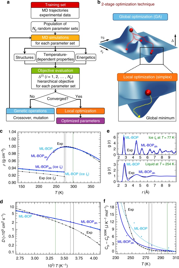
Machine learning protocol to train water potentials and comparison with experiments. a Workflow depicting force field parameterization. One novelty is a direct fitting to dynamically-inferred properties through long time scale MD simulations. N_p refers to population size and Δ⁽ⁱ⁾ refers to errors computed for the i^th parameter set in the N_p population using hierarchical objective. b Diagrams illustrating the 2-stage technique for locating the global minimum of the objective landscape. (The actual optimization involves up to 17 parameters but here we indicate just two generic parameters, α₁ and α₂.) Table 3 has the optimized ML-BOP and ML-BOP_dih parameters. In (c–f) the experimental (Exp) melting point (T = 273 K), maximum density temperature (T = 277 K), and room temperature (T = 298 K) are vertical solid black, dotted black, and solid green lines, respectively. c ML-BOP models accurately reproduce the density anomaly of water within 1.4% as shown by comparison with experimental densities⁵⁵ of ice and liquid water at pressure 1 bar. Melting point of ML-BOP models is 273 ± 1 K. d ML-BOP models predict the experimental diffusion coefficients of water^20,56 over a wide temperature range. e ML-BOP models reproduce the experimental radial distribution functions of ice at T = 77K⁵⁷ and liquid water at T = 254 K²³. f ML-BOP models capture the experimental heat capacity of water⁵⁸ relative to the value at T = 309 K