Abstract
RNA molecules are highly dynamic systems characterized by a complex interplay between sequence, structure, dynamics, and function. Molecular simulations can potentially provide powerful insights into the nature of these relationships. The analysis of structures and molecular trajectories of nucleic acids can be nontrivial because it requires processing very high-dimensional data that are not easy to visualize and interpret. Here we introduce Barnaba, a Python library aimed at facilitating the analysis of nucleic acid structures and molecular simulations. The software consists of a variety of analysis tools that allow the user to (i) calculate distances between three-dimensional structures using different metrics, (ii) back-calculate experimental data from three-dimensional structures, (iii) perform cluster analysis and dimensionality reductions, (iv) search three-dimensional motifs in PDB structures and trajectories, and (v) construct elastic network models for nucleic acids and nucleic acids–protein complexes. In addition, Barnaba makes it possible to calculate torsion angles, pucker conformations, and to detect base-pairing/base-stacking interactions. Barnaba produces graphics that conveniently visualize both extended secondary structure and dynamics for a set of molecular conformations. The software is available as a command-line tool as well as a library, and supports a variety of file formats such as PDB, dcd, and xtc files. Source code, documentation, and examples are freely available at https://github.com/srnas/barnaba under GNU GPLv3 license.
Keywords: MD trajectories, molecular dynamics, RNA 3D structure
INTRODUCTION
Despite their simple four-letter alphabet, RNA molecules can adopt amazingly complex three-dimensional architectures. RNA structure is often described in terms of a few simple degrees of freedom such as backbone torsion angles, sugar puckering, base–base interactions, and helical parameters (Dickerson 1989; Leontis and Westhof 2001; Richardson et al. 2008). Given a known three-dimensional structure, the calculation of these properties can be accurately performed using available tools such as MC-annotate (Gendron et al. 2001), 3DNA (Lu and Olson 2008), fr3D (Sarver et al. 2008), or DSSR (Lu et al. 2015). These software packages allow for a detailed description of experimentally derived RNA structures, but are less suitable for analyzing and comparing large numbers of three-dimensional conformations.
The importance of large-scale analysis tools is critical when considering that many RNA molecules are not static, but highly dynamic entities, and multiple conformations are required to describe their properties. In molecular dynamics (MD) simulations (Šponer et al. 2018), for example, it is often necessary to analyze several hundreds of thousands of structures. The analysis and comparison of results from structure–prediction algorithms poses similar challenges (Dawson and Bujnicki 2016; Magnus 2016; Miao et al. 2017). In order to rationalize and generate scientific insights, it is therefore fundamental to use specific analysis and visualization tools that can handle such highly dimensional data. This need has been long recognized in the field of protein simulations, leading to the development of several software packages for the analysis of MD trajectories (Michaud-Agrawal et al. 2011; McGibbon et al. 2015; Tiberti et al. 2015). While these software packages can be in principle used to analyze generic simulations, they do not support the calculation of nucleic acids-specific quantities out of the box. Notable exceptions are CPPTRAJ (Roe and Cheatham 2013) and the driver tool in PLUMED (Tribello et al. 2014), which support the calculation of nucleic acids structural properties, among other features.
A limited number of software packages have been developed with the main purpose of analyzing simulations of nucleic acids. Curves+ (Lavery et al. 2009) calculates parameters in DNA/RNA double helices as well as torsion backbone angles. dox3dna (Kumar and Grubmüller 2015) extends the capability of the 3DNA package to calculate several base pairs/helical parameters and torsion angles from GROMACS (Abraham et al. 2015) trajectories. The detection of hydrogen bonds/stacking in simulations and the identification of motifs such as helices, junctions, loops, and pseudoknots can be performed using the Motif Identifier for Nucleic acids Trajectory (MINT) software (Górska et al. 2015).
Here we present Barnaba, a Python library to analyze nucleic acid structures and trajectories. The library contains routines to calculate various structural parameters (e.g., distances, torsion angles, base-pair, and base-stacking detection), to perform dimensionality reduction and clustering, to back-calculate experimental quantities from structures, and to construct elastic network models (ENM). Barnaba utilizes the capabilities of MDTraj (McGibbon et al. 2015) for reading/writing trajectory files, and thus supports many different formats, including PDB, dcd, xtc, and trr.
In this paper, we show the capabilities of Barnaba by analyzing a long MD simulation of an RNA stem–loop structure. We first calculate distances from a reference frame. Second, we consider a subset of dihedral angles and compare 3J scalar couplings calculated from simulations with nuclear magnetic resonance (NMR) data. We then perform a cluster analysis of the trajectory, identifying a number of clusters that are visualized using a dynamic secondary structure representation. Finally, we search for structural motifs similar to cluster centroids in the entire protein data bank (PDB) database. In addition, we show how to construct an elastic network model (ENM) of RNA molecules and protein–nucleic acid complexes with Barnaba, and how to use it to estimate RNA local fluctuations. Source code and documentation are freely available at https://github.com/srnas/barnaba under GNU GPLv3 license.
RESULTS
First we provide a list of tools for the analysis of nucleic acid three-dimensional structures supported in Barnaba. All the calculations can be executed from the command-line, as described in Supplemental Material 1. For each functionality, practical examples are provided in Supplemental Material and in the documentation:
Calculate the eRMSD (Bottaro et al. 2014) between structures (Supplemental Material 2).
Calculate the heavy-atom/backbone-only root mean squared distance (RMSD) after optimal superposition (Kabsch 1976) between structures (Supplemental Material 2).
Calculate the relative position and orientations between nucleobases (Supplemental Material 3).
Identify base-pairing and base-stacking interactions in structures and trajectories (Supplemental Material 4).
Calculate backbone, sugar, and pseudorotation torsion angles (Supplemental Material 5).
Back-calculate 3J scalar couplings from structures (Supplemental Material 6).
Search for single-stranded and double-stranded three-dimensional motifs within PDB structures or trajectories (Supplemental Material 7, 8).
Extract fragments with a given sequence from PDB structures. This can be useful to investigate the conformational variability of RNA at a fixed sequence or to perform a stop-motion modeling (SMM) analysis (Supplemental Material 9; Bottaro et al. 2016b).
Perform cluster analysis of RNA structures using the eRMSD (Supplemental Material 10).
Generate “dynamic secondary structure” figures that display the extended secondary structure, together with the population of each interaction within a collection of three-dimensional structures (Supplemental Material 11).
Construct ENM of RNA molecules and protein–nucleic acid complexes (Supplemental Material 12).
Calculate the scoring function eSCORE (Supplemental Material 13; Bottaro et al. 2014; Poblete et al. 2018).
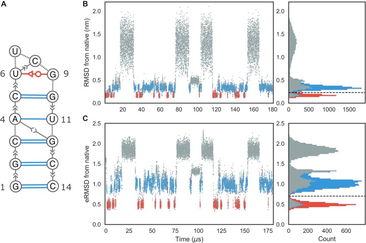
In the following, we present the different features of Barnaba by analyzing a 180 µsec long simulation of an RNA 14-mers with sequence GGCACUUCGGUGCC performed by Tan et al. (2018) using a simulated tempering protocol where the temperature is used as a dynamic variable to enhance sampling. Experimentally, this sequence is known to form an A-form stem composed of five consecutive Watson–Crick base pairs, capped by a UUCG tetraloop (Fig. 1A). In order to make the results described in this paper fully reproducible, we provide in Supplemental Material 14 the Jupyter Notebooks to conduct the analyses and to produce the figures described below.
FIGURE 1.
(A) Extended secondary structure representation of the UUCG stem–loop. Watson–Crick base pairs are shown in blue; trans-Sugar-Watson base pair between U6 and G9 is shown in red. (B) RMSD from native over time of the UUCG simulation. The corresponding histogram is shown in the right panel. The dashed line at RMSD = 0.23 nm separates native-like from nonnative-like structures. The colors indicate the presence of native base–base interactions, as shown in the secondary structure representation. Structures where all Watson–Crick interactions in the stem and the trans-Sugar-Watson base pair in loop are formed are shown in red. Blue indicates structures where only the stem is formed. All other conformations are shown in gray. (C) eRMSD from native structure over time. Color scheme is identical to panel B. Dashed line at eRMSD = 0.7 separates native-like from nonnative conformations.
RMSD, eRMSD calculation, and detection of base–base interactions
We start the analysis by calculating the distance of each frame in the simulation from the reference experimental structure (PDB code 2KOC, Nozinovic et al. 2010) and detecting base–base interactions. Figure 1B shows the time series of heavy-atom RMSD after optimal superposition (Kabsch 1976). During this simulation, multiple folding events occur: In line with previous analyses (Tan et al. 2018), we thus observe both structures close to the reference as well as unfolded/misfolded ones. We identify the base–base interactions in each frame using the annotation functionality in Barnaba (see Materials and Methods). Structures where the stem is completely formed together with the native trans-sugar-Watson (tSW) interaction between U6 and G9 in the loop are shown in red. Blue points indicate structures in which all base pairs in the stem, but not in the loop, are present. All the other structures are colored in gray. From the histogram in Figure 1B, it can be seen that RMSD < 0.23 nm roughly corresponds to native-like structures. A second sharp peak around 0.3 nm corresponds to structures in which only the stem is correctly formed. All other conformations have RMSD larger than 0.6 nm.
One of the features of Barnaba is the possibility to calculate the eRMSD (Bottaro et al. 2014). The eRMSD only considers the relative arrangements between nucleobases in a molecule, and quantifies the differences in the interaction network between two structures. In this perspective, eRMSD is similar to the Interaction Fidelity Network (Parisien et al. 2009) that quantifies the discrepancy in the set of base-pairs and base-stacking interactions. The eRMSD, however, is a continuous, symmetric, positive definite metric distance that satisfies the triangular inequality. Additionally, it does not require detection of the interactions (annotation) and is hence particularly well suited for analyzing MD trajectories and unstructured RNA molecules. Figure 1C shows the eRMSD from native for the UUCG simulation. We notice that, similarly to the RMSD case, the histogram displays three main peaks. In this case, the correspondence between peaks and structures can be readily identified: when eRMSD < 0.7, native stem and loop are formed; if 0.7 < eRMSD < 1.3, stem is formed but the loop is in a nonnative configuration. Other structures typically have eRMSD > 1.3. We observe that the separation between the two main peaks (native structure, red; native stem, blue) is sharper in Figure 1C, confirming that eRMSD is more suitable than RMSD to distinguish structures with different base-pairings (Bottaro et al. 2014).
Note that a significant number of low-RMSD/eRMSD structures lack one or more native base-pair interactions, and are therefore shown in gray. This is because the detection of base–base interactions critically depends on a set of geometrical parameters (e.g., distance, base–base orientation, etc.) that were calibrated on high-resolution structures. The criteria used in Barnaba (as well as the ones used in other annotation tools) may not always be accurate when considering intermediate states and partially formed interactions that are often observed in molecular simulations (Lemieux and Major 2002).
Transition paths
We now analyze the folding/unfolding paths in order to understand what is the nature and order of events leading to folding. In particular, we consider the formation of the native base pairs in the stem and the rotameric state of the χ angle in G9 that is related to the formation of the Sugar-Watson base pair between G9 and U6. Following Lindorff-Larsen et al. (2011), we extract the transition paths (TP) from the simulation, resulting in four folding and four unfolding events. The time evolution for one of the folding events is shown in Figure 2A,B. In the unfolded state, no base pairs are formed and χ freely fluctuates from anti to syn. The three base pairs at the termini form early during the TP, followed by the other two Watson–Crick base pairs. When the native state is reached, all native base pairs are formed, and χ is in syn conformation.
FIGURE 2.
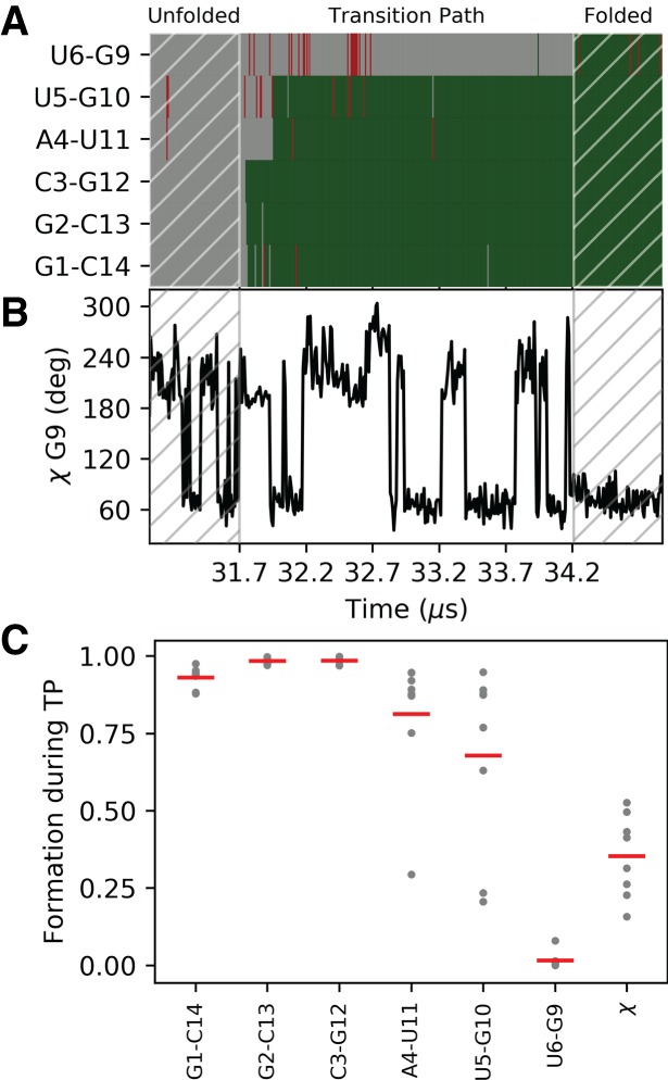
Formation of base pairs and G9-χ angle during RNA folding. (A) Formation of the five WC base pairs over time and of the tSW interaction during one of the folding events. Green indicates that the interaction is formed; gray, not formed. Nonnative interactions are shown in red. (B) Time evolution of the χ angle in G9 for the same folding event shown in panel A. (C) Order of events relative to the formation of the native base pairs and transition to syn. High values correspond to early formation of the corresponding quantity during a folding event. The average over each TP is shown as a gray dot, and the average over the eight TPs is shown as a red bar.
The order of the events can be quantified by calculating the average presence of base pair (assuming values of 1 = formed or 0 = not formed) and the normalized distance from syn conformation q = 0.5(1 + cos (χ − 63°)). Quantities that reach a native-like value (i.e., one) early during folding have a high value, and those that form late get a low value (Lindorff-Larsen et al. 2011). In Figure 2C, we can see that the Watson–Crick 1–14, 2–13, 3–12 form very early in folding, followed by 4–11 and 3–10.The transition of the χ angle to syn occurs at a later stage, and folding is finally achieved with the formation of the tSW base pair.
The TP analysis is here performed for illustrative purposes. In real applications, it is important to take into consideration a number of aspects, such as the quality of the force-field, the assumption that the simulated tempering trajectory is compatible with the real folding pathway, and the employed criteria defining folded/unfolded states (Lindorff-Larsen et al. 2011). Note also that this type of analysis is carried out to describe the properties on the energy barrier, while we here describe the properties of the intermediate state.
Torsion angle and 3J scalar coupling calculations
Another important class of structural parameters is torsion angles. Similarly to other software, Barnaba contains routines to calculate backbone torsion angles (α, β, γ, ε, ζ), the glycosidic angle χ, and the pseudorotation sugar parameters (Altona and Sundaralingam 1972; Rao et al. 1981).
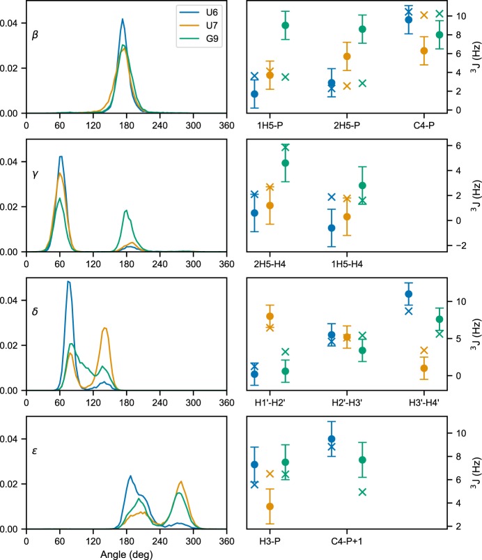
In Figure 3, left panels, we plot the probability distributions of four angles (β, γ, δ, ε) for three different residues: U6, U7, and G9. We can see from the distribution of γ angles that U6 and U7 mainly populate the gauche+ rotameric state (0° < γ ≤ 120°), while G9 significantly populates the trans state as well (120° < γ ≤ 240°). Different rotameric states can also be seen from the distribution of δ angles (C2′/C3′-endo) and ε, which are related to BI/BII states. Here, we consider the same trajectory of the UUCG tetraloops described above and removed all the unfolded structures, i.e., structures with eRMSD from native larger than 1.5 (≈6000 out of 20,000), because we below compare to experiments under conditions where these are absent.
FIGURE 3.
(Left panels) Torsion angle distribution for β, γ, δ, and ε in residues U6, U7, and G9. Right panels show the experimental 3J couplings (crosses) and the calculated value from simulation (dots). The error bars indicate the standard error of the mean calculated over four blocks.
In this example, we chose these specific torsion angles because their distribution is related to available 3J couplings experimental data from NMR spectroscopy. The magnitude of 3J coupling depends on the distance between atoms connected by three bonds, and thus on the corresponding dihedral angle distribution. The dependence between angle θ and coupling 3J can be calculated via Karplus equations:
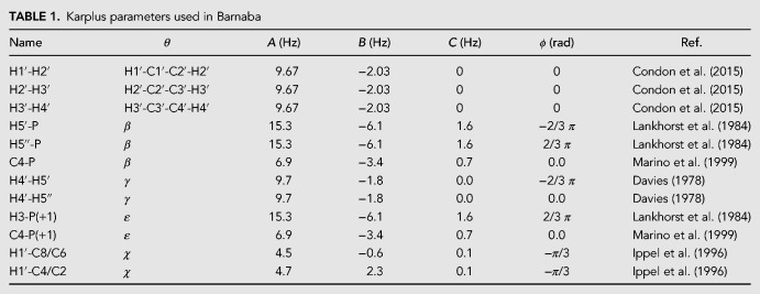
where A, B, C are empirical parameters. Couplings corresponding to different angles can be calculated with Barnaba. H1′-H2′, H2′-H3′, H3′-H4′ (sugar conformation), H5′-P, H5″-P, C4-P (β), H4′-H5′, H4′-H5″ (γ), H3-P(+1), C4-P(+1) (ε), H1′-C8/C6, and H1′-C4/C2 (χ). The complete list of Karplus parameters is reported in the Materials and Methods section, and may be changed within Barnaba.
Figure 3, right panels, shows the back-calculated average 3J couplings and the corresponding experimental value reported in Nozinovic et al. (2010). Note that in some cases, experiments and simulations do not agree: This is because the simulation was performed at different temperatures using a simulated tempering protocol, and therefore the comparison between simulations and experiments is here made for illustrative purposes only. Significant discrepancies could originate from errors introduced by the Karplus equations that can be as large as 2 Hz (Bottaro et al. 2018).
Cluster analysis
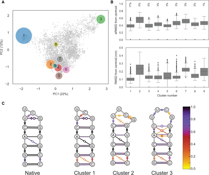
The structures within a trajectory can be grouped into clusters of mutually similar conformations, to understand which different states are visited and how often. For clustering we use the DBSCAN (Ester et al. 1996) algorithm with ε = 0.12 and min samples = 70 (Bottaro and Lindorff-Larsen 2017). As in the previous example, structures with eRMSD > 1.5 from native are discarded. Figure 4A shows the trajectory projected onto the first two components of a principal component analysis done on the collection of G-vectors (Bottaro and Lindorff-Larsen 2017). Circles show the resulting nine clusters, whose radius is proportional to the square root of their size. The 5500 structures (40%) that were not assigned to any cluster are shown as gray dots. For each cluster, we identify its centroid, here defined as the structure with the lowest average distance from all other cluster members.
FIGURE 4.
Example of a cluster analysis on the UUCG stem–loop trajectory. (A) Principal component analysis on the collection of G-vectors (Bottaro and Lindorff-Larsen 2017). Each circle corresponds to a cluster; gray dots show unassigned structures. Circles are centered in the centroid positions, and the radii are proportional to the square root of the population. The percentage of explained variance of the first two components is indicated on the axes. (B) Box-plots reporting eRMSD (top) and RMSD (bottom) from cluster centroids. Lower/upper hinges correspond to the first and third quartiles, while whiskers indicate lowest/highest data within 1.5 interquartile range. Data beyond the end of the whiskers are shown individually. The percentages indicate the cluster population. (C) Dynamic secondary structure representation of the 20 native NMR conformers (PDB 2KOC) and of the first three clusters. The extended secondary structure annotation follows the Leontis–Westhof classification. The color scheme shows the fraction of frames within a cluster for which the interaction is formed.
Ideally, clusters should be compact enough so that the centroid can be considered as a representative structure. This information is shown in the box-plot in Figure 4B, which reports the distances (eRMSD and RMSD, as labeled) between centroids and cluster members. At the same time, structures within clusters are not all identical to one another. In order to visualize the intracluster variability, we have found it useful to introduce a “dynamic secondary structure” representation. In essence, we detect base-stacking/base-pair interactions in all structures within a cluster, and calculate the fraction of frames in which each interaction is present. The population of each interaction is shown by coloring the extended secondary structure representation (Fig. 4C). This representation has some analogy with the “dot plot” representation used to display secondary structure ensembles obtained using nearest neighbor models that reports the predicted probability of individual base pairs (Jacobson and Zuker 1993). We can see that the first three clusters correspond to three different tetraloop structures. In cluster 1, the U6-G9 tSW base pair is present, together with the U6-C8 stacking typical of the native UUCG tetraloop structure. In cluster 2, no U6-G9 base pair is present, while in cluster 3 we observe stacking between U6-U7-C8-G9, as also described in the next section. In all clusters, the population of the terminal base pairs and stacking is lower than one, indicating the presence of base fraying.
In our experience, cluster analysis is useful to understand and qualitatively visualize the different types of structures in a simulation. In many practical cases, however, the number of clusters and their population may differ depending on the employed clustering algorithm and associated parameters. Clustering may not even be meaningful when considering highly unstructured systems such as long single-stranded nucleic acids lacking secondary structures (Chen et al. 2012).
Motif search
Barnaba can be used to search for structural motifs in a PDB file or trajectory using the eRMSD distance. In the following example, we illustrate this feature by taking the centroids of the first three clusters described above and search for similar structures within the PDB database. In order to focus on the loop structure, rather than on stem variability, we consider the tetraloop and the two closing base pairs for the search (residues 4–11 in Fig. 1A). The search is performed against all RNA-containing structures in the PDB database (retrieved May 4, 2018, resolution 3.5 Å or better). The database considered here consists of 3067 X-ray, 652 NMR, and 177 cryo electron-microscopy (EM) structures. Note that the search is purely based on the geometrical arrangement of nucleobases, without restriction on the sequence, a particular feature that is also enabled by the use of eRMSD.
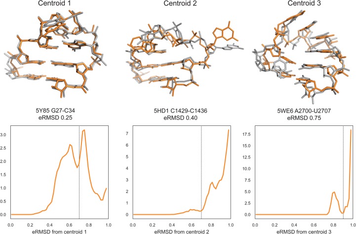
Figure 5 shows the cluster centroids (gray) and the closest motif match, i.e., the lowest eRMSD substructure in the PDB database (orange). The eRMSD between the cluster centroid and the best match are indicated, together with the associated PDB code. Centroid 1 corresponds to the canonical UUCG tetraloop structure, with the signature tSW interaction between U6-G9 and G9 in syn conformation. Note that the eRMSD between centroid and best match is small (0.25), indicating that simulated and experimental structures are highly similar. Cluster 2 corresponds to a structure in which the stem is formed, C8 is stacked on top of U6, and G9 is bulged out. Centroid 3 features four consecutive stackings between U6-U7-C8-G9-G10. Note that this latter structure is remarkably similar to the four-stack loop described in Bottaro and Lindorff-Larsen (2017).
FIGURE 5.
Motif search in PDB database. (Top panels) Centroids of the first three clusters (in gray) superimposed on the closest structures from the PDB database (orange). eRMSD between centroid and the best match are indicated, together with the associated PDB code. (Bottom panels) eRMSD distribution between centroid and substructures from PDB database. Note that different distributions are obtained for different clusters, meaning that the eRMSD threshold varies depending on the motif. Distances larger than eRMSD = 1 are not reported. The eRMSD threshold at 0.7 (centroids 1, 2) and 0.9 (centroid 3) is indicated as a dashed line.
As a rule of thumb, we consider as significant matches structures below 0.7 eRMSD, but there are cases in which it is worth considering structures in the 0.7–1.0 eRMSD range as well. More generally, it is useful to consider the histogram of all fragments with eRMSD below 1, as shown in Figure 5, bottom panels. This type of analysis makes it possible to identify a good threshold value, in correspondence to minima in the probability distributions. For example, there are no structures in the PDB with eRMSD lower than 0.7 for centroid 3. In this case, a value of 0.9 should be used instead.
In this example, we performed a simple search of a structure from simulation against experimentally derived structures in the PDB database. In Barnaba, any arbitrary motif can be used as a query by providing a coordinate file with at least the position of C2, C4, and C6 atoms for each nucleotide. Searches with more complex motifs composed by two strands (e.g., K-turns, sarcin-ricin motifs, etc.) are also possible (Supplemental Material 8). Additionally, Barnaba allows for inserted bases, thereby identifying structural motifs with one or more bulged-out bases.
Elastic network models
Elastic network models (ENMs) are minimal computational models able to capture the dynamics of macromolecules at a small computational cost. They assume that the system can be represented as a set of beads connected by harmonic springs, each having rest length equal to the distance between the two beads it connects in a reference structure (usually, an experimental structure from the PDB). First introduced to analyze protein dynamics (Tirion 1996), ENMs are also applicable to structured RNA molecules (Bahar and Jernigan 1998; Setny and Zacharias 2013; Zimmermann and Jernigan 2014). Barnaba contains routines to construct ENM of nucleic acids and proteins, and, as a unique feature, makes it possible to calculate fluctuations between consecutive C2–C2 atoms. In a previous work (Pinamonti et al. 2015), we have shown this quantity to correlate with flexibility measurements performed with selective 2-hydroxyl acylation analyzed by primer extension (SHAPE) experiments (Merino et al. 2005). Here, we show an example of ENM analysis on two RNA molecules: the 174-nt sensing domain of the Thermotoga maritima lysine riboswitch (PDB ID: 3DIG), and the Escherichia coli 5S rRNA (PDB ID: 1C2X). We construct an all-atom ENM (AA-ENM), where each heavy atom is a bead, together with a cutoff radius of 7 Å. In Figure 6, we show the flexibility of the RNA molecules as predicted by the ENM (black) that can be qualitatively compared with the measured SHAPE reactivity (Hajdin et al. 2013) (orange).
FIGURE 6.
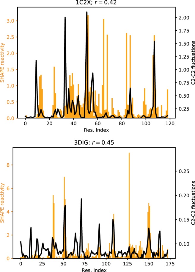
C2–C2 fluctuations as predicted by the ENM of lysine riboswitch (bottom panel) and 5S rRNA (top panel). SHAPE reactivity data from Hajdin et al. (2013) are shown for comparison. Pearson's correlation coefficient r between SHAPE data and ENM-predicted fluctuations is also indicated.
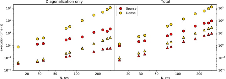
The implementation of the ENM in Barnaba uses the sparse matrix package available in Scipy, which allows for significant speed-ups compared to the dense-matrix implementation. Figure 7 shows the execution time for constructing ENMs of biomolecules with sizes ranging from a few tens to several hundreds of nucleotides. Calculations were performed running Barnaba on a personal computer. This, combined with the significant memory saving granted by sparse matrices representation, makes it possible to easily compute the vibrational modes and the local flexibility of large RNA systems such as ribosomal structures using a limited amount of computer resources.
FIGURE 7.
Execution time for the ENM calculation using sparse matrices (red) or dense matrices (yellow) on a 2.3 GHz Dual-Core Intel Core i5 processor, as a function of the number of residues in the RNA molecule. Results are shown both for sugar-base-phosphate (SBP) ENM (triangles) and all-atom-ENM (AA-ENM) (circles), as defined in Pinamonti et al. (2015). Left panel shows the time for the interaction matrix diagonalization only; right panel shows the total time including the calculation of C2–C2 fluctuations.
DISCUSSION
Many RNA molecules are highly dynamical entities that undergo conformational rearrangements during function. For this reason, it is becoming increasingly important to develop tools to analyze not only single structures, but also trajectories (ensembles) obtained from molecular simulations. In this paper we introduce software to facilitate the analysis of nucleic acids simulations. The program, called Barnaba, is available both as a Python library as well as a command-line tool. The output of the program is such that it can be easily used to calculate averages and probability distributions, or conveniently used as input to the many existing plotting and analysis libraries (e.g., Matplotlib, SKlearn) available in Python.
Barnaba consists of a number of functions, and some of them implement standard calculations (RMSD, torsion angles, base-pairs, and base-stacking detection). A unique feature of Barnaba is the possibility to calculate the eRMSD. This metric has been successfully used in several contexts: for analyzing MD simulations (Kührová et al. 2016), as a biased collective variable in enhanced sampling simulations (Bottaro et al. 2016a; Yang et al. 2017; Poblete et al. 2018), to construct Markov state models (Pinamonti et al. 2017), and to cluster RNA tetraloop structures (Bottaro and Lindorff-Larsen 2017). In this paper we show the usefulness of this metric to monitor simulations over time, to perform cluster analysis, and to search for structural motifs within trajectories/structures. This last feature can be extremely useful to experimental structural biologists, as it makes it possible to efficiently search for arbitrary query motifs within the entire PDB database. For analyzing simulations and clusters, we have found it useful to introduce a dynamic secondary structure representation that recapitulates the variability of base-pair and base-stacking interactions within an ensemble.
Another important feature of Barnaba is the possibility to back-calculate 3J scalar couplings from structures. This calculation is per se extremely simple. However, it can be difficult to obtain from the literature the different sets of Karplus parameters, and the calculation of the corresponding dihedral angles is error-prone.
Finally, Barnaba contains a routine to construct ENMs of nucleic acid and protein systems and complexes. This is a useful, fast, and computationally cheap tool to predict the local dynamical properties of biomolecules, as well as the chain flexibility of RNA molecules.
MATERIALS AND METHODS
Implementation and availability
Barnaba is a Python library and command-line tool. It requires Python 2.7 or >3.3, Numpy, and Scipy libraries. Additionally, Barnaba requires MDTraj (http://mdtraj.org/) for manipulating structures and trajectories. Source code is freely available at https://github.com/srnas/barnaba under GNU GPLv3 license. The github repository contains documentation as well as a set of examples.
Relative position and orientation of nucleobases
For each nucleotide, a local coordinate system is set up in the center of C2, C4, and C6 atoms (Fig. 8). The x-axis points toward the C2 atom, and the y-axis in the direction of C4 (C/U) or C6 (A/G). The origin of the coordinates of nucleobase j in the reference system constructed on base i is the vector Rij = {xij, yij, zij}. Note that |Rij| =|Rji| but Rij ≠Rji. The Rij is central in the definition of the eRMSD metric and of the annotation strategy described below.
FIGURE 8.
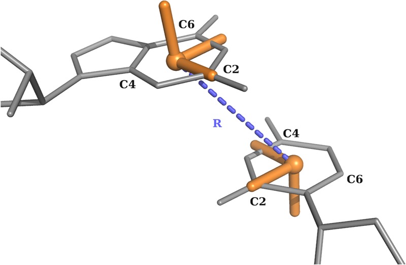
Definition of the local coordinate systems and of the vector R for purines and pyrimidines.
eRMSD
The eRMSD is a contact map-based distance, with the addition of a number of features that make it suitable for the comparison of nucleic acid structures. We briefly describe here the procedure, originally introduced in Bottaro et al. (2014). Given a three-dimensional structure α, one calculates Rijα for all pairs of bases in a molecule. The position vectors are then rescaled as follows:
| (1) |
with a = 5 Å and b = 3 Å. The rescaling effectively introduces an ellipsoidal anisotropy that is peculiar to base–base interactions. Given two structures, α and β, consisting of N residues, the eRMSD is calculated as
| (2) |
G is a nonlinear function of defined as
| (3) |
where and Θ is the Heaviside step function. Note that the function G has the following desirable properties:
.
.
is a continuous function.
The default cutoff value is set to and can be changed within Barnaba.
Annotation
A pair of bases i and j is considered for annotation only if and .
Stacking
The criteria for base stacking are the following:
| (4) |
Here, and θij is the angle between the vectors normal to the planes of the two bases. Similarly to other annotation approaches (Gendron et al. 2001; Sarver et al. 2008; Waleń et al. 2014), we identify four different classes of stacking interactions according to the sign of the z-coordinates:
upward: (≫ or 3′–5′) if zij > 0 and zji < 0
downward: (≪ or 5′–3′) if zij < 0 and zji > 0
outward: (< > or 5′–5′) if zij < 0 and zji < 0
inward: (> < or 3′–3′) if zij > 0 and zji > 0
We notice that, with this choice, consecutive base pairs with alternating purines and pyrimidines result in a cross-strand outward stacking (see, e.g., Fig. 1A).
Base-pairing
Base pairs are classified according to the Leontis–Westhof nomenclature (Leontis and Westhof 2001), based on the observation that hydrogen bonding between RNA bases involves three distinct edges: Watson–Crick (W), Hoogsteeen (H), and sugar (S). An additional distinction is made according to the orientation with respect to the glycosidic bonds, in cis (c) or trans (t) orientation.
In Barnaba, all nonstacked bases are considered base-paired if |θij| < 60° and there exists at least one hydrogen bond, calculated as the number of donor–acceptor pairs with distance <3.3 Å. Edges are defined according to the value of the angle .
Watson-Crick; edge (W): 0.16 < ψ ≤ 2.0 rad
Hoogsteen edge (H): 2.0 < ψ ≤ 4.0 rad
Sugar edge (S): ψ > 4.0rad, ψ ≤ 0.16 rad
These threshold values are obtained by considering the empirical distribution of base–base interactions shown in Supplemental Material 3 and discussed in Figure 2 of Bottaro et al. (2014). Cis/trans orientation is calculated according to the value of the dihedral angle defined by , where N1/N9 is used for pyrimidines and purines, respectively.
We note that the annotation provided by Barnaba might fail in detecting some interactions, and sometimes differs from other programs. This is due to the fact that for non-Watson–Crick and stacking interactions it is not trivial to define a set of criteria for a rigorous discrete classification (Waleń et al. 2014). Typically, these criteria are calibrated to work well for high-resolution structures, but they are not always suitable to describe nearly formed interactions often observed in molecular simulations.
Torsion angles and 3J scalar couplings
We use the standard definition of backbone angles, glycosidic χ angle (O4′-C1′-N9-C4 atoms for A/G, O4′-C1′-N1-C2 for C/U), and sugar torsion angles (ν0 · · · ν4) as shown in Figures 9 and 10 (Saenger 2013).
FIGURE 9.
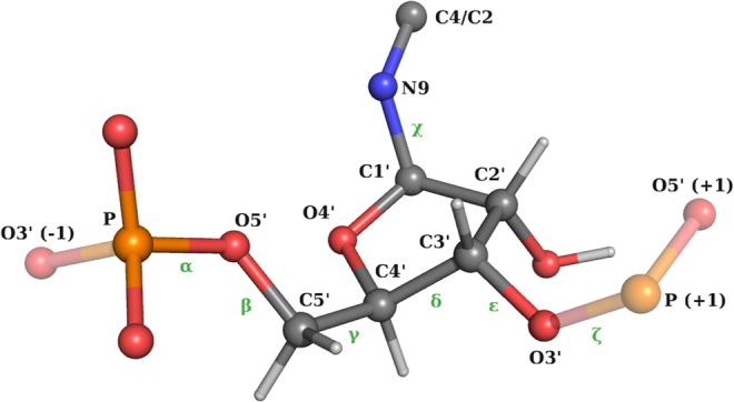
Definition of the backbone/glycosidic angles χ (Frellsen et al. 2009).
FIGURE 10.
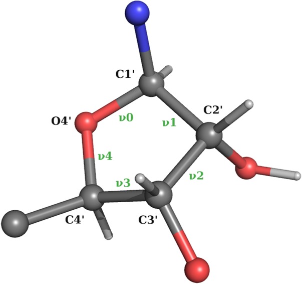
Definition of pucker angles ν0 · · · ν4.
Pseudorotation sugar parameters amplitude tm and phase P are calculated as described in Rao et al. (1981):
| (5) |
| (6) |
where
| (7) |
| (8) |
Optionally, it is also possible to calculate pseudorotation parameters using the Altona–Sundaralingam treatment (Altona and Sundaralingam 1972):
| (9) |
| (10) |
| (11) |
3J Scalar couplings are calculated using the Karplus equations:
| (12) |
Karplus parameters relative to the different scalar couplings are reported in Table 1.
TABLE 1.
Karplus parameters used in Barnaba
Elastic network model
In ENMs, a set of N beads connected by pairwise harmonic springs penalize deviations of interbead distances from their reference values. Spring constants are set to a constant value k whenever the reference distance between the two beads is smaller than an interaction cutoff (Rc), and set to zero otherwise. Under these assumptions, the potential energy of the system can be approximated as
| (13) |
where M is the symmetric 3 N × 3 N interaction matrix, and δri is the deviation of bead i from its position in the reference structure.
The user can select different atoms to be used as beads in the construction of the model. The optimal value of the parameter Rc depends on this choice, as described in Pinamonti et al. (2015).
The covariance matrix is computed as
| (14) |
where λα and vα are the eigenvalues and the eigenvectors of the interaction matrix M, respectively. The sum on α runs over all nonnull modes of the system.
Mean square fluctuation (MSF) of residue i is calculated as
| (15) |
The variance of the distance between two beads can be directly obtained from the covariance matrix in the linear perturbation regime as
| (16) |
where is the µ Cartesian component of the reference distance between beads i and j.
For most practical applications of ENMs, only the high-amplitude modes, i.e., those with the smallest eigenvalues, provide interesting dynamical information. The calculation of C2–C2 distance fluctuations using Equation 16 requires the knowledge of all eigenvectors. This can be performed by reducing the system to the “effective interaction matrix” relative to the beads of interest (Zen et al. 2008).
| (17) |
where MC2(Mother) is formed by the rows and columns of M relative to the (non) C2 beads, while W represent the interactions between C2 and non-C2 beads. The effective interaction matrix is defined as
| (18) |
This can be computed efficiently using sparse matrix-vector multiplication algorithms. The resulting effective matrix has reduced size: 1/3 for sugar-base-phosphate (SBP), ∼1/20 for all-atom (AA), making its pseudo-inversion considerably faster. Note that, in case one is interested in computing the C2–C2 fluctuations for a portion of the molecule only, the algorithm could be further optimized by directly computing the effective interactions matrix associated to the required C2–C2 pairs.
SUPPLEMENTAL MATERIAL
Supplemental material is available for this article.
Supplementary Material
ACKNOWLEDGMENTS
We thank D.E. Shaw Research for providing the simulation of the UUCG tetraloop. The research is funded by a grant from The Velux Foundations (S.B. and K.L.-L.), a Hallas-Møller Stipend from the Novo Nordisk Foundation (K.L.-L.), and the Lundbeck Foundation BRAINSTRUC initiative (K.L.-L.). G.B., S.R., S.B., and G.P. have received funding from the European Research Council (ERC) under the European Union's Seventh Framework Programme (FP/2007-2013)/ERC grant agreement no. 306662 (S-RNA-S). W.B. is funded by Villum Fonden (VKR023445) and the Danish Council for Independent Research (DFF-4181-00344).
Footnotes
Article is online at http://www.rnajournal.org/cgi/doi/10.1261/rna.067678.118.
REFERENCES
- Abraham MJ, Murtola T, Schulz R, Páll S, Smith JC, Hess B, Lindahl E. 2015. GROMACS: high performance molecular simulations through multi-level parallelism from laptops to supercomputers. SoftwareX 1: 19–25. 10.1016/j.softx.2015.06.001 [DOI] [Google Scholar]
- Altona C, Sundaralingam M. 1972. Conformational analysis of the sugar ring in nucleosides and nucleotides. New description using the concept of pseudorotation. J Am Chem Soc 94: 8205–8212. 10.1021/ja00778a043 [DOI] [PubMed] [Google Scholar]
- Bahar I, Jernigan RL. 1998. Vibrational dynamics of transfer RNAs: comparison of the free and synthetase-bound forms. J Mol Biol 281: 871–884. 10.1006/jmbi.1998.1978 [DOI] [PubMed] [Google Scholar]
- Bottaro S, Lindorff-Larsen K. 2017. Mapping the universe of RNA tetraloop folds. Biophys J 113: 257–267. 10.1016/j.bpj.2017.06.011 [DOI] [PMC free article] [PubMed] [Google Scholar]
- Bottaro S, Di Palma F, Bussi G. 2014. The role of nucleobase interactions in RNA structure and dynamics. Nucleic Acids Res 42: 13306–13314. 10.1093/nar/gku972 [DOI] [PMC free article] [PubMed] [Google Scholar]
- Bottaro S, Banáš P, Šponer J, Bussi G. 2016a. Free energy landscape of GAGA and UUCG RNA tetraloops. J Phys Chem Lett 7: 4032–4038. 10.1021/acs.jpclett.6b01905 [DOI] [PubMed] [Google Scholar]
- Bottaro S, Gil-Ley A, Bussi G. 2016b. RNA folding pathways in stop-motion. Nucleic Acids Res 44: 5883–5891. 10.1093/nar/gkw239 [DOI] [PMC free article] [PubMed] [Google Scholar]
- Bottaro S, Bussi G, Kennedy SD, Turner DH, Lindorff-Larsen K. 2018. Conformational ensembles of RNA oligonucleotides from integrating NMR and molecular simulations. Sci Adv 4: eaar8521 10.1126/sciadv.aar8521 [DOI] [PMC free article] [PubMed] [Google Scholar]
- Chen H, Meisburger SP, Pabit SA, Sutton JL, Webb WW, Pollack L. 2012. Ionic strength-dependent persistence lengths of single-stranded RNA and DNA. Proc Natl Acad Sci 109: 799–804. 10.1073/pnas.1119057109 [DOI] [PMC free article] [PubMed] [Google Scholar]
- Condon DE, Kennedy SD, Mort BC, Kierzek R, Yildirim I, Turner DH. 2015. Stacking in RNA: NMR of four tetramers benchmark molecular dynamics. J Chem Theory Comput 11: 2729–2742. 10.1021/ct501025q [DOI] [PMC free article] [PubMed] [Google Scholar]
- Davies DB. 1978. Conformations of nucleosides and nucleotides. Prog NMR Spectrosc 12: 135–225. 10.1016/0079-6565(78)80006-5 [DOI] [Google Scholar]
- Dawson WK, Bujnicki JM. 2016. Computational modeling of RNA 3D structures and interactions. Curr Opin Struct Biol 37: 22–28. 10.1016/j.sbi.2015.11.007 [DOI] [PubMed] [Google Scholar]
- Dickerson R. 1989. Definitions and nomenclature of nucleic acid structure components. Nucleic Acids Res 17: 1797–1803. 10.1093/nar/17.5.1797 [DOI] [PMC free article] [PubMed] [Google Scholar]
- Ester M, Kriegel HP, Sander J, Xu X. 1996. A density-based algorithm for discovering clusters in large spatial databases with noise. KDD 96: 226–231. [Google Scholar]
- Frellsen J, Moltke I, Thiim M, Mardia KV, Ferkingho-Borg J, Hamelryck T. 2009. A probabilistic model of RNA conformational space. PLoS Comput Biol 5: e1000406 10.1371/journal.pcbi.1000406 [DOI] [PMC free article] [PubMed] [Google Scholar]
- Gendron P, Lemieux S, Major F. 2001. Quantitative analysis of nucleic acid three-dimensional structures. J Mol Biol 308: 919–936. 10.1006/jmbi.2001.4626 [DOI] [PubMed] [Google Scholar]
- Górska A, Jasiński M, Trylska J. 2015. MINT: software to identify motifs and short-range interactions in trajectories of nucleic acids. Nucleic Acids Res 43: e114 10.1093/nar/gkv559 [DOI] [PMC free article] [PubMed] [Google Scholar]
- Hajdin CE, Bellaousov S, Huggins W, Leonard CW, Mathews DH, Weeks KM. 2013. Accurate SHAPE-directed RNA secondary structure modeling, including pseudoknots. Proc Natl Acad Sci 110: 5498–5503. 10.1073/pnas.1219988110 [DOI] [PMC free article] [PubMed] [Google Scholar]
- Ippel J, Wijmenga S, De Jong R, Heus H, Hilbers C, De Vroom E, Van der Marel G, Van Boom J. 1996. Heteronuclear scalar couplings in the bases and sugar rings of nucleic acids: their determination and application in assignment and conformational analysis. Magn Reson Chem 34: S156–S176. [DOI] [Google Scholar]
- Jacobson AB, Zuker M. 1993. Structural analysis by energy dot plot of a large mRNA. J Mol Biol 233: 261–269. 10.1006/jmbi.1993.1504 [DOI] [PubMed] [Google Scholar]
- Kabsch W. 1976. A solution for the best rotation to relate two sets of vectors. Acta Crystallogr A 32: 922–923. 10.1107/S0567739476001873 [DOI] [Google Scholar]
- Kührová P, Best RB, Bottaro S, Bussi G, Šponer J, Otyepka M, Banáš P. 2016. Computer folding of RNA tetraloops: identification of key force field deficiencies. J Chem Theory Comput 12: 4534–4548. 10.1021/acs.jctc.6b00300 [DOI] [PMC free article] [PubMed] [Google Scholar]
- Kumar R, Grubmüller H. 2015. do_x3dna: a tool to analyze structural fluctuations of dsDNA or dsRNA from molecular dynamics simulations. Bioinformatics 31: 2583–2585. 10.1093/bioinformatics/btv190 [DOI] [PubMed] [Google Scholar]
- Lankhorst PP, Haasnoot CA, Erkelens C, Altona C. 1984. Carbon-13 NMR in conformational analysis of nucleic acid fragments. 2. A reparametrization of the Karplus equation for vicinal NMR coupling constants in CCOP and HCOP fragments. J Biomol Struct Dyn 1: 1387–1405. 10.1080/07391102.1984.10507527 [DOI] [PubMed] [Google Scholar]
- Lavery R, Moakher M, Maddocks JH, Petkeviciute D, Zakrzewska K. 2009. Conformational analysis of nucleic acids revisited: Curves+. Nucleic Acids Res 37: 5917–5929. 10.1093/nar/gkp608 [DOI] [PMC free article] [PubMed] [Google Scholar]
- Lemieux S, Major F. 2002. RNA canonical and non-canonical base pairing types: a recognition method and complete repertoire. Nucleic Acids Res 30: 4250–4263. 10.1093/nar/gkf540 [DOI] [PMC free article] [PubMed] [Google Scholar]
- Leontis NB, Westhof E. 2001. Geometric nomenclature and classification of RNA base pairs. RNA 7: 499–512. 10.1017/S1355838201002515 [DOI] [PMC free article] [PubMed] [Google Scholar]
- Lindorff-Larsen K, Piana S, Dror RO, Shaw DE. 2011. How fast-folding proteins fold. Science 334: 517–520. 10.1126/science.1208351 [DOI] [PubMed] [Google Scholar]
- Lu XJ, Olson WK. 2008. 3DNA: a versatile, integrated software system for the analysis, rebuilding and visualization of three-dimensional nucleic-acid structures. Nat Protoc 3: 1213–1227. 10.1038/nprot.2008.104 [DOI] [PMC free article] [PubMed] [Google Scholar]
- Lu XJ, Bussemaker HJ, Olson WK. 2015. DSSR: an integrated software tool for dissecting the spatial structure of RNA. Nucleic Acids Res 43: e142 10.1093/nar/gkv716 [DOI] [PMC free article] [PubMed] [Google Scholar]
- Magnus M. 2016. rna-pdb-tools: a toolbox to analyze structures and simulations of RNA. http://rna-pdb-tools.rtfd.io [Google Scholar]
- Marino JP, Schwalbe H, Griesinger C. 1999. J-coupling restraints in RNA structure determination. Acc Chem Res 32: 614–623. 10.1021/ar9600392 [DOI] [Google Scholar]
- McGibbon RT, Beauchamp KA, Harrigan MP, Klein C, Swails JM, Hernández CX, Schwantes CR, Wang LP, Lane TJ, Pande VS. 2015. MDTraj: a modern open library for the analysis of molecular dynamics trajectories. Biophys J 109: 1528–1532. 10.1016/j.bpj.2015.08.015 [DOI] [PMC free article] [PubMed] [Google Scholar]
- Merino EJ, Wilkinson KA, Coughlan JL, Weeks KM. 2005. RNA structure analysis at single nucleotide resolution by selective 2′-hydroxyl acylation and primer extension (SHAPE). J Am Chem Soc 127: 4223–4231. 10.1021/ja043822v [DOI] [PubMed] [Google Scholar]
- Miao Z, Adamiak RW, Antczak M, Batey RT, Becka AJ, Biesiada M, Boniecki MJ, Bujnicki JM, Chen SJ, Cheng CY, et al. 2017. RNA-Puzzles Round III: 3D RNA structure prediction of five riboswitches and one ribozyme. RNA 23: 655–672. 10.1261/rna.060368.116 [DOI] [PMC free article] [PubMed] [Google Scholar]
- Michaud-Agrawal N, Denning EJ, Woolf TB, Beckstein O. 2011. MDAnalysis: a toolkit for the analysis of molecular dynamics simulations. J Comput Chem 32: 2319–2327. 10.1002/jcc.21787 [DOI] [PMC free article] [PubMed] [Google Scholar]
- Nozinovic S, Fürtig B, Jonker HR, Richter C, Schwalbe H. 2010. High-resolution NMR structure of an RNA model system: the 14-mer cUUCGg tetraloop hairpin RNA. Nucleic Acids Res 38: 683–694. 10.1093/nar/gkp956 [DOI] [PMC free article] [PubMed] [Google Scholar]
- Parisien M, Cruz JA, Westhof E, Major F. 2009. New metrics for comparing and assessing discrepancies between RNA 3D structures and models. RNA 15: 1875–1885. 10.1261/rna.1700409 [DOI] [PMC free article] [PubMed] [Google Scholar]
- Pinamonti G, Bottaro S, Micheletti C, Bussi G. 2015. Elastic network models for RNA: a comparative assessment with molecular dynamics and SHAPE experiments. Nucleic Acids Res 43: 7260–7269. 10.1093/nar/gkv708 [DOI] [PMC free article] [PubMed] [Google Scholar]
- Pinamonti G, Zhao J, Condon DE, Paul F, Noé F, Turner DH, Bussi G. 2017. Predicting the kinetics of RNA oligonucleotides using Markov state models. J Chem Theory Comput 13: 926–934. 10.1021/acs.jctc.6b00982 [DOI] [PMC free article] [PubMed] [Google Scholar]
- Poblete S, Bottaro S, Bussi G. 2018. A nucleobase-centered coarse-grained representation for structure prediction of RNA motifs. Nucleic Acids Res 46: 1674–1683. 10.1093/nar/gkx1269 [DOI] [PMC free article] [PubMed] [Google Scholar]
- Rao S, Westhof E, Sundaralingam M. 1981. Exact method for the calculation of pseudorotation parameters P, τm and their errors. A comparison of the Altona–Sundaralingam and Cremer–Pople treatment of puckering of five-membered rings. Acta Crystallogr A 37: 421–425. 10.1107/S0567739481000892 [DOI] [Google Scholar]
- Richardson JS, Schneider B, Murray LW, Kapral GJ, Immormino RM, Headd JJ, Richardson DC, Ham D, Hershkovits E, Williams LD, et al. 2008. RNA backbone: consensus all-angle conformers and modular string nomenclature (an RNA Ontology Consortium contribution). RNA 14: 465–481. 10.1261/rna.657708 [DOI] [PMC free article] [PubMed] [Google Scholar]
- Roe DR, Cheatham TE III. 2013. PTRAJ and CPPTRAJ: software for processing and analysis of molecular dynamics trajectory data. J Chem Theory Comput 9: 3084–3095. 10.1021/ct400341p [DOI] [PubMed] [Google Scholar]
- Saenger W. 2013. Principles of nucleic acid structure. Springer Science & Business Media, New York. [Google Scholar]
- Sarver M, Zirbel CL, Stombaugh J, Mokdad A, Leontis NB. 2008. FR3D: finding local and composite recurrent structural motifs in RNA 3D structures. J Math Biol 56: 215–252. 10.1007/s00285-007-0110-x [DOI] [PMC free article] [PubMed] [Google Scholar]
- Setny P, Zacharias M. 2013. Elastic network models of nucleic acids flexibility. J Chem Theory Comput 9: 5460–5470. 10.1021/ct400814n [DOI] [PubMed] [Google Scholar]
- Šponer J, Bussi G, Krepl M, Banáš P, Bottaro S, Cunha RA, Gil-Ley A, Pinamonti G, Poblete S, Jurečka P, et al. 2018. RNA structural dynamics as captured by molecular simulations: a comprehensive overview. Chem Rev 118: 4177–4338. 10.1021/acs.chemrev.7b00427 [DOI] [PMC free article] [PubMed] [Google Scholar]
- Tan D, Piana S, Dirks RM, Shaw DE. 2018. RNA force field with accuracy comparable to state-of-the-art protein force fields. Proc Natl Acad Sci 115: E1346–E1355. 10.1073/pnas.1713027115 [DOI] [PMC free article] [PubMed] [Google Scholar]
- Tiberti M, Papaleo E, Bengtsen T, Boomsma W, Lindorff-Larsen K. 2015. ENCORE: software for quantitative ensemble comparison. PLoS Comput Biol 11: e1004415 10.1371/journal.pcbi.1004415 [DOI] [PMC free article] [PubMed] [Google Scholar]
- Tirion MM. 1996. Large amplitude elastic motions in proteins from a single-parameter, atomic analysis. Phys Rev Lett 77: 1905–1908. 10.1103/PhysRevLett.77.1905 [DOI] [PubMed] [Google Scholar]
- Tribello GA, Bonomi M, Branduardi D, Camilloni C, Bussi G. 2014. PLUMED 2: new feathers for an old bird. Comp Phys Commun 185: 604–613. 10.1016/j.cpc.2013.09.018 [DOI] [Google Scholar]
- Waleń T, Chojnowski G, Gierski P, Bujnicki JM. 2014. ClaRNA: a classifier of contacts in RNA 3D structures based on a comparative analysis of various classification schemes. Nucleic Acids Res 42: e151 10.1093/nar/gku765 [DOI] [PMC free article] [PubMed] [Google Scholar]
- Yang C, Lim M, Kim E, Pak Y. 2017. Predicting RNA structures via a simple van der Waals correction to an all-atom force field. J Chem Theory Comput 13: 395–399. 10.1021/acs.jctc.6b00808 [DOI] [PubMed] [Google Scholar]
- Zen A, Carnevale V, Lesk AM, Micheletti C. 2008. Correspondences between low-energy modes in enzymes: dynamics-based alignment of enzymatic functional families. Protein Sci 17: 918–929. 10.1110/ps.073390208 [DOI] [PMC free article] [PubMed] [Google Scholar]
- Zimmermann MT, Jernigan RL. 2014. Elastic network models capture the motions apparent within ensembles of RNA structures. RNA 20: 792–804. 10.1261/rna.041269.113 [DOI] [PMC free article] [PubMed] [Google Scholar]
Associated Data
This section collects any data citations, data availability statements, or supplementary materials included in this article.


