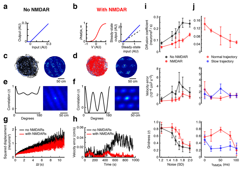
Figure 5. Active dendrites in MECII neurons can enhance the robustness of the rate code of grid cell firing.

(a,b) CAN model simulations were performed either in the absence (a) or the presence (b) of a slow supralinear integration mechanism, as provided by NMDARs (τ_NMDA = 50 ms). (c,d) Left: animal trajectory (blue; data from Hafting et al.¹²) and CAN network prediction of animal position in the absence (c) (black) or in the presence (d) (red) of NMDARs are superimposed. Right: color-coded spatial rate maps for an example model neuron in the absence (c) or in the presence (d) of NMDARs. (e,f) Left: correlation between rotated autocorrelation maps plotted against the rotation angle. Simulations were performed in the absence (e) or in the presence (f) of NMDARs. Right: autocorrelation matrices of the spatial rate maps shown in c and d, respectively. (g) To quantify network drift, mean squared displacement is plotted as a function of simulation time interval in the absence of velocity inputs in the absence (black) or in the presence (red) of NMDARs. (h) Absolute difference between animal velocity and optimally scaled network velocity plotted against time in the absence (black) or in the presence (red) of NMDARs. (i) From top to bottom: network diffusion coefficient in the absence of velocity inputs, summed squared velocity error and gridness, each plotted against noise s.d. for CAN network simulations with (red symbols) or without (black symbols) NMDARs. (j) The same quantities as in i plotted against τ_NMDA. Simulations were performed using either the original animal trajectory (red symbols) or a version that was slowed by a factor of 2 (blue symbols). In the simulations in a–h, noise s.d. = 1.6, and error bars represent s.e.m. of 7 simulations, which were initialized with different pseudorandom number generator seeds.