Figure - PMC

Skip to main content

An official website of the United States government

Here's how you know

Here's how you know

Official websites use .gov
A .gov website belongs to an official government organization in the United States.

Secure .gov websites use HTTPS
A lock ( ) or https:// means you've safely connected to the .gov website. Share sensitive information only on official, secure websites.

View full-text article in PMC

. 2019 Feb 4;9:1328. doi: 10.1038/s41598-018-36675-8

Search in PMC
Search in PubMed
View in NLM Catalog
Add to search

© The Author(s) 2019

Open Access This article is licensed under a Creative Commons Attribution 4.0 International License, which permits use, sharing, adaptation, distribution and reproduction in any medium or format, as long as you give appropriate credit to the original author(s) and the source, provide a link to the Creative Commons license, and indicate if changes were made. The images or other third party material in this article are included in the article’s Creative Commons license, unless indicated otherwise in a credit line to the material. If material is not included in the article’s Creative Commons license and your intended use is not permitted by statutory regulation or exceeds the permitted use, you will need to obtain permission directly from the copyright holder. To view a copy of this license, visit http://creativecommons.org/licenses/by/4.0/.

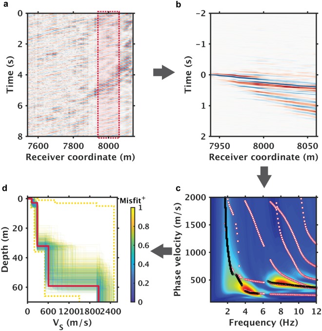
PMC Copyright notice

Illustration of data processing workflow for ambient noise interferometry. (a) Example of train noise shown via an 8 second time domain slice. The red box in (a) highlights subsection of the array used for (b) noise correlation gather, (c) dispersion analysis, and (d) inversion of the shear-wave velocity (V_S) profiles. Black and white markers in (c) denote observed and model-predicted multimodal dispersion curves respectively. In (d), the yellow dashed lines denote upper and lower bounds of the parameter space used in Monte Carlo sampling; the bold red line marks the best-fit V_S profile; the yellow/blue lines denote the top 0.1% best-fitting V_S profiles (color coded by their corresponding inversion misfits); Misfit^† denotes normalized misfit values (min-max normalized by misfits of the top 0.1% V_S profiles).