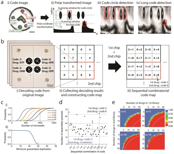
Figure 3.

The automatic decoding and statistical analysis of code distributions. a) Decoding algorithm. (i) “Long code,” “short code,” and “code circles” are components for identifying the rotation, inversion, and code number of microparticles, respectively. Scale bar: 30 µm. (ii)–(iv) Particle image is transformed into polar coordinates, and the locations of each code component are recognized by a machine‐learning‐based algorithm. b) Construction of sequential combinatorial code map. Decoding results from all images are collected, and a sequential combinatorial code map is generated. c) Probability about the minimum duplication number. (i) Probabilities that a “specific” combination has a duplicate greater than n according to the number of microwells. (ii) Probability that “all” combinations will be found over a certain number of duplicates in 1600 microwells. d) Example of combinatorial code distribution. First and second drug libraries contain four and eight kinds of drugs, respectively. Total 45 combinations (including single or no drug treatment, represented by blue dots) were found from 1600 microwells. Red line (n = 32) is the expected value except for the cases in which no particle is applied in the second treatment (blue dots). e) Available library size for sequential combination screening in a single chip (1600 microwells). Color represents the probability of partipetting to guarantee that all combinations have duplications greater than n. White dashed lines are available library size for conventional pipetting technique.