A deep learning approach for human behavior prediction with explanations in health social networks: social restricted Boltzmann machine (SRBM⁺)

Abstract

Human behavior modeling is a key component in application domains such as healthcare and social behavior research. In addition to accurate prediction, having the capacity to understand the roles of human behavior determinants and to provide explanations for the predicted behaviors is also important. Having this capacity increases trust in the systems and the likelihood that the systems will be actually adopted, thus driving engagement and loyalty. However, most prediction models do not provide explanations for the behaviors they predict. In this paper, we study the research problem, human behavior prediction with explanations, for healthcare intervention systems in health social networks. In this work, we propose a deep learning model, named social restricted Boltzmann machine (SRBM), for human behavior modeling over undirected and nodes-attributed graphs. In the proposed SRBM⁺ model, we naturally incorporate self-motivation, implicit and explicit social influences, and environmental events together. Our model not only predicts human behaviors accurately, but also, for each predicted behavior, it generates explanations. Experimental results on real-world and synthetic health social networks confirm the accuracy of SRBM⁺ in human behavior prediction and its quality in human behavior explanation.

1. Introduction

Human behavior modeling normally requires a predictive mechanism that can predict a future behavior of an individual, such as click, a buy, a call, or exercise. It can take the observed attributes of the individual and the social network as input and provide a predictive score as output. The higher the score, the more likely the individual will exhibit the predicted behavior. Given its open-ended nature, the application domains of human behavior prediction are very broad, e.g., healthcare, politics, e-commerce, psychology, personal life, financial risk, etc. (Siegel 2013). However, the challenge is that most prediction models do not provide explanations for the behaviors they predict (i.e., why the specific, predicted behaviors are more likely). Providing explanations for human behaviors is even more important than only providing the prediction, itself, in most applications (Freitas 2014). This is well understood in many areas, such as human computing, biology and medicine, psychology and social sciences, e-commerce, online social networks, etc. (Freitas 2014; Siegel 2013).

In this paper, we study the research problem of human behavior prediction with explanations in the application of healthcare intervention for overweight and obese people through online social networks. To reduce the risk of obesity-related diseases (e.g., diabetes, cardiovascular diseases, cancers), interventions such as regular exercise are strongly recommended (Pate et al. 1995). Many intervention systems have been developed to engage people to exercise regularly. The Internet is identified as an important source of health information, and it may thus be an appropriate delivery vector for health behavior interventions (Marshall et al. 2005). In addition, mobile devices can track and record the walking/jogging/running distance and intensity of an individual. Our recent study, conducted in 2010–2011 as a collaboration between a PeaceHealth Laboratories, SK Telecom Americas, and University of Oregon, utilized these technologies to record daily physical activities, social activities (i.e., text messages, social games, events, competitions, etc.), biomarkers, and biometric measures (i.e., cholesterol, triglyceride, BMI, etc.) for a group of 254 overweight and obese individuals. All users enrolled in a health social network allowing them to befriend and communicate with each other. Users’ biomarkers and biometric measures were recorded via daily, weekly, or monthly medical tests performed at home (individually) or at our laboratories.

Our starting observation is that human behavior is the outcome of interacting determinants such as self-motivation, social influences, and environmental events. This observation is rooted in sociology and psychology, where it is referred to as human agency in social cognitive theory (Bandura 1989). An individual’s self-motivation can be captured by learning correlations between his or her historic and current attributes. Modeling social influences in social networks is challenging, since they are categorized into implicit and explicit social influences (Christakis 2010). Explicit social influences are influences on user behavior derived from direct connections in a health social network. This is insufficient, however, to fully characterize social influences. Distinct from explicit social influences, implicit social influences (Christakis 2010) are the accumulated effects of limited information regarding users’ social activities, changing social context, and influence derived from unacquainted users participating in a common social activity. The effects of environmental events on users’ behaviors can be captured by learning the correlations between off-line events and users’ attributes.

Modeling human behaviors in a health social network with explanations has the benefit to increase the trust in the intervention. It targets the intervention approaches to specific and truthful problems to keep the users maintaining or improving their health status, and thus to increase the successful adaptation rate. However, human behavior explanation in the context of healthcare intervention systems is still widely underdeveloped. In this paper, we propose a novel social restricted Boltzmann machine model for human behavior explanation (SRBM⁺), which not only predicts human behaviors accurately, but also, for each predicted behavior, it can generate an insightful explanation. The SRBM⁺ model quantifies the implicit social influences by incorporating temporal dependencies of individuals on social communities and personal representation together. The implicit social influences on an individual is an aggregation function of the past of the health social network. Similarly, the self-motivation is an aggregation function of his/her historical representation. In addition, we define a new temporal smoothing and statistical function to capture explicit social influences on individuals from their friends. By combining implicit and explicit social influences into a linear adaptive bias, we are able to model and explain the social influences. The environmental events such as competitions, meet-ups, and social games are integrated into the model as observed variables, which will directly affect the outcome of user behaviors. Finally, our SRBM⁺ model provides a natural way to statistically estimate the effects of human behavior determinants, which are used to generate explanations for predicted behaviors by using state-of-the-art interpretable classifiers (Bien and Tibshirani 2011; Breiman et al. 1984; Fung et al. 2005; Meinshausen 2010; Van Assche and Blockeel 2007). Our main contributions are as follows:

• We study the research problem of human behavior prediction with explanations in health social networks, which is motivated by real-world healthcare intervention systems.

• We introduce SRBM⁺, a novel deep learning model which can accurately predict and explain human behaviors.

• An extensive experiment conducted on real-world and synthetic health social networks confirms the high prediction accuracy and quality of generated explanations of our model.

In Sect. 2, we introduce the RBM and related works. We describe our health social network in Sect. 3. The social restricted Boltzmann machine (SRBM⁺) model for human behavior prediction with explanations is in Sect. 4. The experimental evaluation is in Sect. 5, and we conclude the paper in Sect. 6.

2. The RBMs and related works

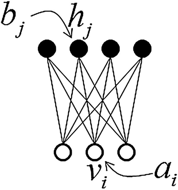
The restricted Boltzmann machine (RBM) (Smolensky 1986) is a deep learning structure that has a layer of visible units fully connected to a layer of hidden units but no connections within a layer (Fig. 1). Typically, RBMs use stochastic binary units for both visible and hidden variables.

Fig. 1.

The RBM

To model real-valued data, a modified RBM with binary logistic hidden units and real-valued Gaussian visible units can be used. In Fig. 1, v_i and h_j are, respectively, used to denote the states of visible unit i and hidden unit j. a_i and b_j are used to distinguish biases on the visible and hidden units. The RBM assigns a probability to any joint setting of the visible units, v and hidden units, h:

$$p\left(v,h\right)=\frac{\text{exp}\left(-E\left(v,h\right)\right)}{Z}$$ (1)

where E(v, h) is an energy function,

$$E\left(v,h\right)={\displaystyle \sum }_i\frac{{\left(v_i-a_i\right)}^2}{2{\xi }_i^2}-{\displaystyle \sum }_j{b}_j{h}_j-{\displaystyle \sum }_{ij}\frac{v_i}{{\xi }_i}{h}_j{W}_{ij}$$ (2)

where ξ_i is the standard deviation of the Gaussian noise for visible unit i. In practice, fixing ξ_i at 1 makes the learning work well. Z is a partition function which is intractable as it involves a sum over the exponential number of possible joint configurations: Z = Σ_v′,h′ E(v′, h′). The conditional distributions (with ξ_i = 1) are:

$$p\left(h_j=1|v\right)=\sigma \left(b_j+{\displaystyle \sum }_i{v}_i{W}_{ij}\right)$$ (3)

$$p\left(v_i|h\right)=\mathcal{N}\left(a_i+{\displaystyle \sum }_j{h}_j{W}_{ij},1\right)$$ (4)

where σ(.) is a logistic function, and $\mathcal{N}\left(\mu ,V\right)$ is a Gaussian.

Given a training set of state vectors, the weights and biases in an RBM can be learned following the gradient of contrastive divergence. The learning rules are:

$$\begin{gathered} \Delta W_{ij}={\langle v_i{h}_j\rangle }_d-{\langle v_i{h}_j\rangle }_r \\ \Delta b_{ij}={\langle h_j\rangle }_d-{\langle h_j\rangle }_r \end{gathered}$$ (5)

where the first expectation 〈.〉_d. is based on the data distribution and the second expectation 〈.〉_r is based on the distribution of ‘‘reconstructed’’ data.

To incorporate temporal dependencies into the RBM, the CRBM (Taylor et al. 2006) adds autoregressive connections from the visible and hidden variables of an individual to his/her historical variables. The CRBM simulates well human motion in the single agent scenario. However, it cannot capture the social influences on individual behaviors in the multiple agent scenario. Li et al. (2014) proposed the ctRBM model for link prediction in dynamic networks. The ctRBM simulates the social influences by adding the prediction expectations of local neighbors on an individual into a dynamic bias. However, the visible layer of the ctRBMs does not take individual attributes as input. Thus, the ctRBM cannot directly predict human behaviors.

Meanwhile, social behavior has been studied recently, such as analysis of user interactions in Facebook (Viswanath et al. 2009), activity recommendation (Lerman et al. 2012), and user activity level prediction (Shen et al. 2012; Zhu et al. 2013). In Zhu et al. (2013), the authors focus on predicting users who have a tendency to lower their activity levels. This problem is known as churn prediction. Churn prediction aims to find users who will leave a network or a service. By finding such users, service providers could analyze the reasons and figure out the strategies to maintain such users in different applications, including online social games (Kawale et al. 2009), QA forum (Yang et al. 2010), etc. In Shen et al. (2012), proposed two types of human behavior prediction methods: personalized behavior prediction methods and socialized behavior prediction methods. Personalized methods only leverage individuals’ past behavior records for future behavior predictions. Socialized methods use both one person’s past behavior records and his or her friends’ past behaviors for predictions. Specifically, five models reported in Shen et al. (2012) are socialized Gaussian process (SGP) model, socialized logistical autoregression (SLAR) model, personalized Gaussian process (PGP) model, logistical autoregression (LAR) model, and behavior pattern search (BPS) model. The main weak point of these methods is: They are either lacking of the ability to take into account multiple individual features, e.g., BMI, messages, physical activities, (SGP, PGP, BPS) or laking of the ability to efficiently capture social correlations and social influences (SLAR, LAR). Our focus is to address all these challenging issues. In addition, our goal is not only to predict, but also to understand the roles of human behavior determinants, and to give explanations for predicted behaviors. In Barbieri et al. (2014), the authors provide the WTFW model, which generates explanations for user-to-user links, but not for human behaviors.

This paper is an extension of our conference paper published in ASONAM 2015 (Phan et al. 2015). The major extensions we have engaged are: (1) We have improved our previous SRBM model not only so that it more accurately predicts human behavior, but also, it can generate explanations for each predicted behavior. We introduce a new social influence function by incorporating physical activity-based social influence into our previous SRBM model, a new algorithm to quantitatively estimate the effects and roles of human behavior determinants in predicted behaviors. (2) An extensive experiment has been conducted on both real-world and synthetic health social networks to validate the effectiveness of our model, the roles of human behavior determinants, and the quality of generated explanations.

3. YesiWell health social network

In the previous section, we have quickly reviewed the RBMs and related works, including extended versions of traditional RBMs and state-of-the-art human behavior prediction models. In this section, we will present our YesiWell health social network in detail.

Our health social network data was collected from Oct 2010 to Aug 2011, as a collaboration between PeaceHealth Laboratories, SK Telecom Americas, and University of Oregon, to record daily physical activities, social activities (i.e., text messages, competitions, etc.), biomarkers, and biometric measures (i.e., cholesterol, BMI, etc.) for a group of 254 individuals. Physical activities, including measurements of the number of walking and running steps, were reported every 15 min via a mobile device carried by each user. As mentioned in our Introduction, all users enrolled in an online social network, allowing them to befriend and communicate with each other. Users’ biomarkers and biometric measures were recorded via daily/weekly/monthly medical tests performed at home (i.e., individually) or at our laboratories. In total, we have approximately over 7 million data points of physical exercise, over 21,205 biomarker and biometric measurements, 1371 friend connections, and 2766 inbox messages. Our longitudinal study was conducted for 10 months. Albeit that such might seem a short interval, when compared with public social networks, i.e., Twitter and Facebook, our health social network is a unique, solid, and comprehensive multi-dimensional social network. The YesiWell network contains rich information from social activities, physical activities, and biomarkers and biometric measures, availing us unique access to verify statements about physical activity with recorded physical activity, and to compare statements about health with clinical measures of health.

In this paper, 33 features are taken into account (Table 1). All the features are summarized daily and weekly. The features are designed to capture the self-motivation of each user. Some of the key measures are as follows:

Table 1.

Personal attributes

Behaviors	#joining competitions #goals achieved #meet-up	#exercising days ∑ (distances) #social games	#goals set avg (speeds)
Social communications (the number of inbox messages)	Encouragement	Fitness	Followup
	Competition	Games	Personal
	Study protocol	Progress report	Technique
	Social network	Meet-ups	Goal
	Wellness meter	Feedback	Heckling
	Explanation	Invitation	Notice
	Technical fitness	Physical
Biomarkers	Wellness score	BMI	BMI slope
	Wellness score slope

• Personal ability BMI, fitness, cholesterol, etc.

• Attitudes the number of off-line events in which each user participates, individual sending and receiving messages, the number of goals set and achieved, Wellness score (Kil et al. 2012), etc. Wellness score is a measure to evaluate how well a user lives their life. Being active in social activities, setting and achieving more goals, and getting higher wellness score illustrate a healthier attitude of a user.

• Intentions the number of competitions each user joins, the number of goals set, etc. We measure intent to exercise in terms of competitions joined and goals set.

• Effort the number of exercise days, walking/running steps, the distances, and speed walked/run.

• Withdrawal the increase of BMI slope and/or decrease of Wellness score (Kil et al. 2012) indicates negative signs in the self-motivation. Users may give up.

The ability to learn hidden correlations among multiple individual features is crucial to capture self-motivation in different contexts. In the next section, we will present our model to learn the joint representation of self-motivation, social influence, and environmental events for human behavior prediction with explanations.

4. Human behavior prediction with explanations

In this section, we first present our SRBM⁺ model for human behavior prediction in our YesiWell health social network, then explanations will be generated based on our predictive model. Given our health social network, denoted as $G=\left\{U,E,\mathcal{F}\right\}$ where U is a set of all users, each user has a set of individual attributes $\mathcal{F}=\left\{f_1,\dots ,f_n\right\}$. The social network G grows from scratch over a set of time points T = {t₁, …, t_m}. To illustrate this, we use $E=\left\{E_{t_1},\dots ,E_{t_m}\right\}$ to denote the topology of the network G over time, where E_t is a set of edges (i.e., friend connections) which have been made until time t in the network, and ∀t ∈ T : E_t ⊆ E_t+1. For each user, the values of individual attributes in $\mathcal{F}$ also change over time. We denote the values of individual attributes of a user u at time t as ${\mathcal{F}}_u^t$. At each time point t, each user u is associated with a binomial behavior $y_u^t\in \left\{0,1\right\}\cdot y_u^t$ could be ‘‘decrease’’ or ‘‘increase’’ exercise. We will describe $y_u^t$ more clearly in our experimental result section.

Problem formulation Given the health social network G in M timestamps T_data = {t – M + 1, …, t} we want to predict the behavior of all the users in the next timestamp t + 1. Formally, given $\left\{{\mathcal{F}}_u^t,y_u^t,E_t|t\in T_{\text{data}},u\in U\right\}$ we predict $\left\{y_u^{t+1}|u\in U\right\}$.

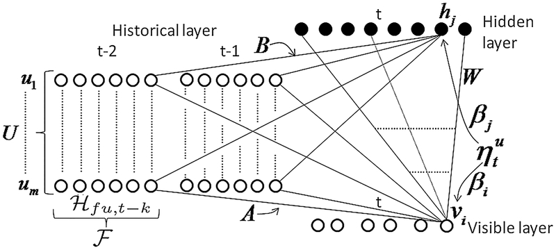
Figure 2 illustrates the proposed SRBM⁺ model. The structure of human behavior modeling includes three layers: visible layer v, hidden layer h, and historical layer $\mathcal{H}$. Given a user, each visible variable v_i in the visible layer v corresponds to an individual feature f_i at time t. All the visible variables of all the users in the previous N time intervals {t – N, …, t – 1} (i.e., N < M) are included in a historical layer, denoted by ${\mathcal{H}}_{t<}$. In addition, the variables in the historical layer are called historical variables. Obviously, we will have $\left|\mathcal{F}\right|\times \left|U\right|\times N$ historical variables. The hidden layer h consists of |h| hidden variables. The challenge is to connect the three layers together and model the variables to capture human behavior determinants.

Fig. 2.

The social restricted Boltzmann machine (SRBM⁺) model

4.1. Self-motivation

Self-motivation is composed of many dimensions including attitudes, intentions, effort, belief, and withdrawal, any and all of which can affect the motivation that an individual experiences (Ryan and Deci 2000). In order to model self-motivation of a user u, we first fully connect the hidden and visible layers via a weight matrix W (Fig. 2). Then each visible variable v_i and hidden variable h_j will be connected to all the historical variables of u, denoted by ${\mathcal{H}}_{fu,t-k}$ where $f\in \mathcal{F}$ and k ∈ {1, …, N} These connections are presented by the two weight matrices A and B (Fig. 2). Each historical variable ${\mathcal{H}}_{fu,t-k}$ is the state of feature f of the user u at time poin t − k. Note that all the historical variables are treated as additional observed inputs. Since the attributes are designed to reflect self-motivation, the effect of his/her past attributes captures the self-motivation of user u. This effect can be integrated into dynamic biases of each hidden variable h_j and visible variable v_i:

$${\widehat{b}}_{j,t}=b_j+{\displaystyle \sum }_{k\in \left\{1,\dots ,N\right\}}{\displaystyle \sum }_{f\in \mathcal{F}}{B}_{jfu,t-k}{\mathcal{H}}_{fu,t-k}$$ (6)

$${\widehat{a}}_{i,t}=a_i+{\displaystyle \sum }_{k\in \left\{1,\dots ,N\right\}}{\displaystyle \sum }_{f\in \mathcal{F}}{A}_{ifu,t-k}{\mathcal{H}}_{fu,t-k}$$ (7)

which include static biases b_j and a_i, and the contribution from the past of the user u.B_j and A_i are |h| × |U| × N and |v| × |U| × N weight matrices which summarize the autoregressive parameters to the hidden and visible variable h_j; v_i. This modifies the factorial distribution over hidden and visible variables: b_j; a_i in Eqs. 3 and 4 are replaced with ${\widehat{b}}_{j,t},{\widehat{a}}_{i,t}$ to obtain

$$p\left(h_{j,t}=1|v_t,{\mathcal{H}}_{t<}\right)=\sigma \left({\widehat{b}}_{j,t}+{\displaystyle \sum }_i{v}_{i,t}{W}_{ij}\right)$$ (8)

$$p\left(v_{i,t}|h_t,{\mathcal{H}}_{t<}\right)=\sigma \left({\widehat{a}}_{i,t}+{\displaystyle \sum }_j{v}_{j,t}{W}_{ij},1\right)$$ (9)

where h_j,t is the state of hidden variable j at time t, the weight W_ij connects v_i and h_j.

4.2. Implicit social influences and environmental events

The implicit social influences are composed of unobserved social relationships, unacquainted users, and the changing of social context (Christakis 2010). It is hard to exactly define implicit social influences. Fortunately, the dynamics of neural networks offer us a great solution toward capturing the flexibility of implicit social influences. In fact, given a user u, each visible variable v_i and hidden variable h_j are connected to all historical variables of all other users. This is similar to the self-motivation modeling: the influence effects of each user, and the social context on the user u, are captured via the weight matrices A and B. Thus, these effects can be integrated into the dynamic biases ${\widehat{a}}_{i,t}$ and ${\widehat{b}}_{j,t}$ as well. The dynamic biases in Eqs. 6 and 7 become:

$${\widehat{b}}_{j,t}=b_j+{\displaystyle \sum }_{k\in \left\{1,\dots ,N\right\}}{\displaystyle \sum }_{f\in \mathcal{F}}{\displaystyle \sum }_{u\in U}{B}_{jfu,t-k}{\mathcal{H}}_{fu,t-k}$$ (10)

$${\widehat{a}}_{i,t}=a_i+{\displaystyle \sum }_{k\in \left\{1,\dots ,N\right\}}{\displaystyle \sum }_{f\in \mathcal{F}}{\displaystyle \sum }_{u\in U}{A}_{ifu,t-k}{\mathcal{H}}_{fu,t-k}$$ (11)

The environmental events, such as the number of competitions, meet-up events, and social games, are included as individual attributes. Therefore, the effect of environmental events is well embedded into the model. That effect will interact with self-motivation and implicit social influences to capture the behaviors of the users. Next, we will incorporate the explicit social influence into our model.

4.3. Explicit social influences

It is well known that individuals tend to be friends with people who perform behaviors similar to theirs (homophily principle). In addition, as shown in Phan et al. (2014), users differentially experience and absorb physical exercise-based influences from their friends. Therefore, the explicit social influences in health social networks can be defined as a function of the homophily effect and physical exercise-based social influences. Let us first define user similarity as follows.

Given two neighboring users u and m, a simple way to quantify their similarity is to applying a cosine function of their individual representations (i.e., v^u and v^m) and hidden features (i.e., h^u and h^v). The user similarity between u and m at time t, denoted s_t(u, m), is defined as:

$$s_t\left(u,m\right)={\text{cos}}_t\left(u,m|v\right)\times {\text{cos}}_t\left(u,m|h\right)$$ (12)

where cos_t(.) is a cosine similarity function, i.e.,

$${\text{cos}}_t\left(u,m|v\right)=\frac{p\left(v_t^u|h_t^u,{\mathcal{H}}_{t<}^u\right)\cdot p\left(v_t^m|h_t^m,{\mathcal{H}}_{t<}^m\right)}{\parallel p\left(v_t^u|h_t^u,{\mathcal{H}}_{t<}^u\right)\parallel \parallel p\left(v_t^m|h_t^m,{\mathcal{H}}_{t<}^m\right)\parallel }$$

$${\text{cos}}_t\left(u,m|h\right)=\frac{p\left(h_t^u|v_t^u,{\mathcal{H}}_{t<}^u\right)\cdot p\left(h_t^m|v_t^m,{\mathcal{H}}_{t<}^m\right)}{\parallel p\left(h_t^u|v_t^u,{\mathcal{H}}_{t<}^u\right)\parallel \parallel p\left(h_t^m|v_t^m,{\mathcal{H}}_{t<}^m\right)\parallel }$$

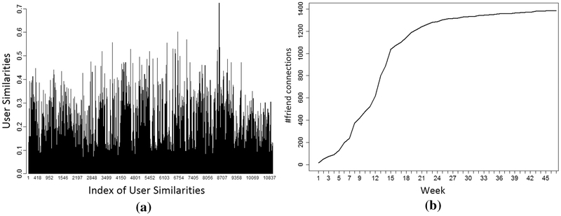
Figure 3a illustrates a sample of a user similarity spectrum of all the edges in our social network over time. We randomly select 35 similarities of neighboring users for each day in ten months. Apparently, the distributions are not uniform, and different time intervals present various distributions. To well qualify the similarity between individuals and their friends, it potentially requires a cumulative distribution function (CDF). In addition, our health social network is developed from scratch. As time goes by, each participant will have more connections to other users (Fig. 3b). Thus a temporal smoothing is needed to better capture the explicit social influences. Eventually, we propose a statistical explicit social influence, denoted ${\eta }_t^u$, of a user u at time t as follows:

$${\eta }_t^u=\alpha {\eta }_{t-\tau }^u+\left(1-\alpha \right)\frac{1}{\left|{\mathbb{F}}_t^u\right|}{\displaystyle \sum }_{m\in {\mathbb{F}}_t^u}{\psi }_t\left(m,u\right)\times p\left(s_t\le s_t\left(u,m\right)\right)$$

where ${\mathbb{F}}_t^u$ is a set of friends of user u until time t from the beginning. ψ_t(m, u) is the physical exercise-based social influence m on u at time t, which is derived by using the CPP model (Phan et al. 2014). s_t is the similarity between two arbitrary neighboring users in the social network at time t. p (s_t ≤ s_t(u, m)) represents the probability that the similarity is less than or equal to the instant similarity s_t(u, m). α and τ are two parameters to control the dynamics of η.

Fig. 3.

A sample of cosine similarities (a) and cumulative number of friend connections (b) in our dataset

4.4. Inference, learning, and prediction

Inference in the SRBM⁺ is no more difficult than in the RBM. The states of the hidden variables are determined both by the inputs they receive from the visible variables and from the historical variables. The conditional probability of hidden variables at time interval t can be computed as in Eqs. 6 and 8. The combination of the implicit and explicit social influences can be viewed as a linear adaptive bias: ${\widehat{a}}_{i,t}$ in Eq. 7 becomes

$${\widehat{a}}_{i,t}=a_i+{\displaystyle \sum }_{k\in \left\{1,\dots ,N\right\}}{\displaystyle \sum }_{f\in \mathcal{F}}{\displaystyle \sum }_{u\in U}{A}_{ifu,t-k}{\mathcal{H}}_{fu,t-k}+{\beta }_i{\eta }_t^u$$

$${\widehat{b}}_{j,t}=b_j+{\displaystyle \sum }_{k\in \left\{1,\dots ,N\right\}}{\displaystyle \sum }_{f\in \mathcal{F}}{\displaystyle \sum }_{u\in U}{B}_{jfu,t-k}{\mathcal{H}}_{fu,t-k}+{\beta }_j{\eta }_t^u$$

where β_i is a parameter which presents the ability to observe the explicit social influences ${\eta }_t^u$ of user u given v_i.

The energy function becomes:

$$E\left(v_t,h_t|{\mathcal{H}}_{t<},\theta \right)={\displaystyle \sum }_{i\in v}\frac{{\left(v_{i,t}-{\widehat{a}}_{i,t}\right)}^2}{2{\xi }_i^2}-{\displaystyle \sum }_{j\in h}{\widehat{b}}_{j,t}{h}_{j,t}-{\displaystyle \sum }_{i\in v,j\in h}\frac{v_{i,t}}{{\xi }_i}{h}_{j,t}{W}_{ij}+\lambda |\theta =\left\{A,B,W,\beta \right\}{|}_1$$

Contrastive divergence is used to train the SRBM⁺ model. The updates for the symmetric weights, W, the static biases, a and b, the directed weights, A and B, are based on simple pairwise products. The gradients are summed over all the training time intervals t ∈ T_train = T_data\{t – M + 1, …, t – M + N}. The learning rules are summarized in Table 2.

Table 2.

Learning rules

Algorithm	Learning rules
Contrastive divergence	$\Delta W_{ij}={\sum }_t\left({\langle v_{i,t}{h}_{j,t}\rangle }_d-{\langle v_{i,t}{h}_{j,t}\rangle }_r\right)$
	$\Delta a_i={\sum }_t\left({\langle v_{i,t}\rangle }_d-{\langle v_{i,t}\rangle }_r\right)$
	$\Delta b_j={\sum }_t\left({\langle h_{j,t}\rangle }_d-{\langle h_{j,t}\rangle }_r\right)$
	$\Delta A_{ifu,t-k}={\sum }_t\left({\langle v_{i,t}{\mathcal{H}}_{fu,t-k}\rangle }_d-{\langle v_{i,t}{\mathcal{H}}_{fu,t-k}\rangle }_r\right)$
	$\Delta B_{jfu,t-k}={\sum }_t\left({\langle h_{j,t}{\mathcal{H}}_{fu,t-k}\rangle }_d-{\langle h_{f,t}{\mathcal{H}}_{fu,t-k}\rangle }_r\right)$
	$\Delta {\beta }_i={\sum }_t\left({\langle v_{i,t}\rangle }_d-{\langle v_{i,t}\rangle }_r\right){\eta }_t^u$
	$\Delta {\beta }_j={\sum }_t\left({\langle h_{j,t}\rangle }_d-{\langle h_{j,t}\rangle }_r\right){\eta }_t^u$
Back-propagation	$\frac{\partial C\left(\theta \right)}{\partial s_j}=-{\sum }_t\left(y_1-{\widehat{y}}_t\right)h_j$
	$\frac{\partial C\left(\theta \right)}{{\partial }_c}=-{\sum }_t\left(y_1-{\widehat{y}}_t\right)$
	$\frac{\partial C\left(\theta \right)}{\partial W_{ij}}=-{\sum }_t\left(y_1-{\widehat{y}}_t\right)s_j{h}_j\left(1-h_j\right)v_i$
	$\frac{\partial C\left(\theta \right)}{\partial a_i}=-{\displaystyle {\sum }_t\left(y_1-{\widehat{y}}_t\right)s_j{h}_j\left(1-h_j\right)W_{ij}}$
	$\frac{\partial C\left(\theta \right)}{\partial b_j}=-{\displaystyle {\sum }_t\left(y_1-{\widehat{y}}_t\right)s_j{h}_j\left(1-h_j\right)}$
	$\frac{\partial C\left(\theta \right)}{\partial A_{ifu,t-k}}=-{\displaystyle {\sum }_t\left(y_1-{\widehat{y}}_t\right)s_j{h}_j\left(1-h_j\right)W_{ij}{\mathcal{H}}_{fu,t-k}}$
	$\frac{\partial C\left(\theta \right)}{\partial B_{jfu,t-k}}=-{\displaystyle {\sum }_t\left(y_1-{\widehat{y}}_t\right)s_j{h}_j\left(1-h_j\right){\mathcal{H}}_{fu,t-k}}$
	$\frac{\partial C\left(\theta \right)}{\partial {\beta }_i}=-{\displaystyle {\sum }_t\left(y_1-{\widehat{y}}_t\right)s_j{h}_j\left(1-h_j\right)W_{ij}{\eta }_t^u}$
	$\frac{\partial C\left(\theta \right)}{\partial b_j}=-{\displaystyle {\sum }_t\left(y_1-{\widehat{y}}_t\right)s_j{h}_j\left(1-h_j\right){\eta }_t^u}$

On top of our model, we put an output layer for the user behavior prediction task. Our goal is to predict whether a user increases or decreases physical exercise levels. Thus the softmax layer contains a single output variable $\widehat{y}$ and binary target values: 1 for increases, and 0 for decreases. The output variable $\widehat{y}$ is fully linked to the hidden variables by weighted connections S, which includes |h| parameters s_j. The logistic function is used as an activation function of $\widehat{y}$ as follows:

$$\widehat{y}=\sigma \left(c+{\displaystyle \sum }_{j\in h}{h}_j{s}_j\right)$$

where c is a static bias. Given a user u ∈ U, a set of training vectors $X=\left\{{\mathcal{F}}_u^t,E_t|t\in T_{\text{train}}\right\}$, and an output vector Y = {y_t|t ∈ T_train}, the probability of a binary output y_t ∈ {0, 1} given input x_t is as follows:

$$P\left(Y|X,\theta \right)={\displaystyle \prod }_{t\in T_{\text{train}}}{\widehat{y}}_t^{y_t}{\left(1-{\widehat{y}}_t\right)}^{1-y_t}$$ (13)

where ${\widehat{y}}_t=P\left(y_t=1|x_t,\theta \right)$.

A loss function to appropriately deal with the binomial problem is cross-entropy error. It is given by

$$C\left(\theta \right)=-{\displaystyle \sum }_{t\in T_{\text{train}}}\left(y_t\text{log}{\widehat{y}}_t+\left(1-y_t\right)\text{log}\left(1-{\widehat{y}}_t\right)\right)$$ (14)

In the final stage of training, Back-propagation is used to fine-tune all the parameters together. The derivatives of the objective C(θ) with respect to all the parameters over all the training cases t ∈ T_train are summarized in Table 2. In the prediction task, we need to predict the $y_u^{t+1}$ without observing the ${\mathcal{F}}_u^{t+1}$. In other words, the visible and hidden variables are not observed at the future time point t + 1. Thus we need a causal generation step to initiate these variables. Causal generation from a learned SRBM⁺ model can be done just like the learning procedure. In fact, we always keep the historical variables fixed and perform alternating Gibbs sampling to obtain a joint sample of the visible and hidden variables from the SRBM⁺ model. To start alternating Gibbs sampling, a good choice is to set v_t = v_t−1, (i.e., v_t−1 is a strong prior of v_t). This picks new hidden and visible variables that are compatible with each other and with the recent historical variables. Afterward, we aggregate the hidden variables to evaluate the output $\widehat{y}$.

4.5. Explanation generation

We have presented our human behavior prediction model, our training process, and our inference algorithm in the previous section. In this section, our focus is to generate explanations for each predicted behavior.

The success of human behavior intervention does not only depend on its accuracy in inferring and exploring users’ behaviors, but it also relies on how the deployed interventions are perceived by the users. Explanations increase the transparency of the intervention process and contribute to users’ satisfaction, and in engaging users to the program. When generating explanations for human behaviors, the first step is to quantitatively estimate the causal roles of human behavior determinants in the predicted behaviors. The SRBM⁺ model provides a natural way to address this. The effects of human behavior determinants are reflected via the ways we formulate the dynamic biases. To evaluate the effect of self-motivation on predicted behaviors, we compute the output variable ${\widehat{y}}_{t+1}$ by using the dynamic biases ${\widehat{b}}_{j,t}$ and ${\widehat{a}}_{i,t}$ which are in the forms of Eqs. 6 and 7. This means we only use the self-motivation effect to predict the behaviors of the users. Similarly, we can evaluate the effects of implicit social influences, explicit social influences, and environmental events. The corresponding dynamic biases for each human behavior determinant are summarized in Table 3. We use ${\widehat{y}}_{t+1,\text{self}},{\widehat{y}}_{t+1,\text{im}},{\widehat{y}}_{t+1,\text{ex}}$, and ${\widehat{y}}_{t+1,\text{env}}$ to denote the output variable ${\widehat{y}}_t$ given corresponding determinants. With regard to the effect of environmental events, we use the number of joined competitions, meet-up events, and social games to evaluate the output variable ${\widehat{y}}_{t+1,\text{env}}$.

Table 3.

Dynamic biases of human behavior determinants

Determinants (output variable)	Dynamic biases
Self-motivation $\left({\widehat{y}}_{t+1,\text{self}}\right)$	${\widehat{b}}_{j,t}=b_j+{\displaystyle {\sum }_{k=1}^N{\displaystyle {\sum }_{f\in \mathcal{F}}{B}_{jfu,t-k}{\mathcal{H}}_{fu,t-k}}}$
	${\widehat{a}}_{i,t}=a_i+{\displaystyle {\sum }_{k=1}^N{\displaystyle {\sum }_{f\in \mathcal{F}}{A}_{ifu,t-k}{\mathcal{H}}_{fu,t-k}}}$
Implicit social influence $\left({\widehat{y}}_{t+1,\text{im}}\right)$	${\widehat{b}}_{j,t}=b_j+{\displaystyle {\sum }_{k=1}^N{\displaystyle {\sum }_{f\in \mathcal{F}}{\displaystyle {\sum }_{\underset{m\ne u}{m\in U}}{B}_{jfm,t-k}{\mathcal{H}}_{fm,t-k}}}}$
	${\widehat{a}}_{i,t}=a_i+{\displaystyle {\sum }_{k=1}^N{\displaystyle {\sum }_{f\in \mathcal{F}}{\displaystyle {\sum }_{\underset{m\ne u}{m\in U}}{B}_{ifm,t-k}{\mathcal{H}}_{fm,t-k}}}}$
Explicit social influence $\left({\widehat{y}}_{t+1,\text{ex}}\right)$	${\widehat{b}}_{j,t}=b_j+{\beta }_j{\eta }_t^u$
	${\widehat{a}}_{i,t}=a_i+{\beta }_i{\eta }_t^u$
Environmental events $\left({\widehat{y}}_{t+1,\text{env}}\right)$	only use #competitions,#meet-up events, #social games in the SRBM+ model

We can then generate explanations for the predicted behavior based on ${\widehat{y}}_{t+1,\text{self}},{\widehat{y}}_{t+1,\text{im}},{\widehat{y}}_{t+1,\text{ex}}$ and ${\widehat{y}}_{t+1,\text{env}}$ by using state-of-the-art, interpretable classifiers. The algorithms used in this paper are 1-nearest neighbors, decision trees (Breiman et al. 1984), node harvest (NH) (Meinshausen 2010), Ism_td (Van Assche and Blockeel 2007), ExtractedRules-PCM (Fung et al. 2005), and prototype selection (PS) (Bien and Tibshirani 2011). To avoid losing information when applying decision trees, NH, and Ism_td algorithms, we will use the output variables ${\widehat{y}}_{t+1}$ instead of the binary predicted behaviors (i.e., 1 iff ${\widehat{y}}_{t+1}>.05$, otherwise 0). To do this we modify the entropy of a training set as follows: for a training set containing p users whose predicted behaviors are ‘1’ and q users whose predicted behaviors are ‘0,’ the entropy can be defined as

$$H\left(p,q\right)=-\frac{P}{P+Q}{\text{log}}_2\frac{P}{P+Q}-\frac{Q}{P+Q}{\text{log}}_2\frac{Q}{P+Q}$$ (15)

where $P={\sum }_{u\in p}{\widehat{y}}_{t+1}^u$ and $Q={\sum }_{v\in q}\left(1-{\widehat{y}}_{t+1}^u\right),{\widehat{y}}_{t+1}^u$ and ${\widehat{y}}_{t+1}^u$ are the output variables of u, v at time t + 1.

There are several other interpretable classifiers reported in Freitas (2014). However, many of them cannot be directly applied in our work. For instance, we need to discretize our numerical attributes without golden standards before applying interpretable linear classifiers by Ustun and Rudin (Ustun and Rudin 2014).

5. Experimental results

We have carried out a series of experiments in a real health social network to validate our proposed SRBM⁺ model (source codes and data).¹ We first elaborate about the experiment configurations, evaluation metrics, and baseline approaches. Then, we introduce the experimental results.

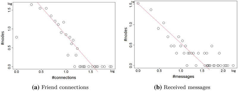
Experiment configurations In our study, we take into account 33 personal attributes (Table 1). The personal social communications include 2766 inbox messages, which are categorized into 20 different types. Figure 4 illustrates the distributions of friend connections, and #received messages in our data. They clearly follow the Power law distribution. Note that, given a week, if a user exercises more than his/her last week, he/she is considered to be increasing exercise; otherwise, the user will be considered to be decreasing exercise. The number of hidden units, and the number of previous time intervals N, respectively, are set to 200 and 3. In the individual representation learning, the number of hidden units at all the concepts and sub-concepts in the ontology will double the number of visible units. The weights are randomly initialized from a zero-mean Gaussian with a standard deviation of 0.01. All the learning rates are set to 10⁻³. A contrastive divergence CD₂₀ is used to maximize likelihood learning. We train the model for each user independently.

Fig. 4.

Some distributions in our dataset

Evaluation metrics In the experiment, we leverage the previous 10 weeks’ records to predict the behaviors of all the users (i.e., increase or decrease exercises) in the next week. The prediction quality metric, i.e., accuracy, is as follows:

$$\text{accuracy}=\frac{{\displaystyle \sum {}_{i=\mathrm{1..}\left|U\right|}I\left(y_i={\widehat{y}}_i\right)}}{\left|U\right|}$$

where y_i is the true user activity of the user u_i, and ${\widehat{y}}_i$ denotes the predicted value, I is the indication function.

Competitive prediction models We compare the SRBM⁺ model with the conventional methods reported in Shen et al. (2012). The competitive methods are divided into two categories: personalized behavior prediction methods and socialized behavior prediction methods. Personalized methods only leverage individuals’ past behavior records for future behavior predictions. Socialized methods use both one person’s past behavior records and his or her friends’ past behaviors for predictions. Specifically, five models reported in Shen et al. (2012) are socialized Gaussian process (SGP) model, socialized logistical autoregression (SLAR) model, personalized Gaussian process (PGP) model, Logistical autoregression (LAR) model, and Behavior Pattern Search (BPS) model.

We also consider the RBM related extensions, i.e., the CRBM (Taylor et al. 2006) and ctRBM (Li et al. 2014), as competitive models. The CRBM can be directly applied to our problem by ignoring the implicit and explicit influences in our SRBM⁺ model. Since the ctRBM cannot directly incorporate individual attributes with social influences to model human behaviors, we only can apply its social influence function into our model. In fact, we replace our statistical explicit social influence function by the ctRBM’s social influence function. We call this version of ctRBM a Socialized ctRBM (SctRBM). We also compare the SRBM⁺ model with our previous work, in Phan et al. (2015).

5.1. Validation of the SRBM⁺ Model for Prediction

Our task of validation focuses on three key issues: (1) which configurations of the parameters α and τ produce the best-fit social influence distribution, (2) which of the potential social influence functions and our statistical explicit social function produce a better-fit social influence distribution, and (3) whether the SRBM⁺ model is better than the competitive models in terms of prediction accuracy. We carry out the validation through three approaches. One is to conduct human behavior prediction with various settings of α and τ. By this we look for an optimal configuration for the statistical explicit social influence function. The second validation is to compare the optimal setting of our statistical explicit social influence function with its different forms and existing algorithms. The third validation is to compare our SRBM⁺ model with the competitive models in terms of prediction accuracy.

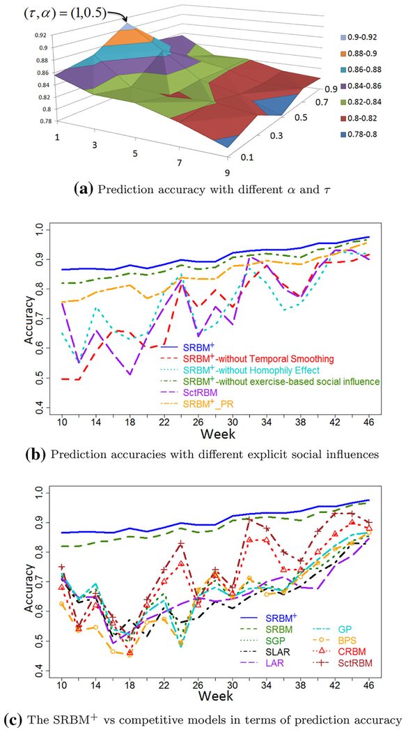
Figure 5a illustrates the surface of the prediction accuracy of the SRBM⁺ model with variations of the two parameters α and τ on our health social network. We observed that the smaller values of τ tend to have higher prediction accuracies. This is quite reasonable since the more recent behaviors have stronger influences. The temporal smoothing parameter τ has similar effects to a time decay function (Zhu et al. 2013). Meanwhile, the middle range values of α offer better prediction accuracies. Clearly, the optimal setting values of α and τ are 0.5 and 1 respectively.

Fig. 5.

Validation of the SRBM⁺ model

To test the correctness, we compare our optimal setting (i.e., τ = 1. α = 0.5) of the explicit social influence function with its different forms, such as: (1) without the temporal smoothing component, i.e., ${\eta }_t^u=\frac{1}{\left|{\mathbb{F}}_t^u\right|}{\sum }_{m\in {\mathbb{F}}_t^u}{\psi }_t\left(m,u\right)\times p\left(s_t\le s_t\left(u,m\right)\right)$, (2) without the homophily effect, i.e., ${\eta }_t^u=\alpha {\eta }_{t-1}^u+\left(1-\alpha \right)\frac{1}{\left|{\mathbb{F}}_t^u\right|}{\sum }_{m\in {\mathbb{F}}_t^u}{\psi }_t\left(m,u\right)$, (3) without physical exercise-based social influence, i.e., ${\eta }_t^u=\frac{1}{\left|{\mathbb{F}}_t^u\right|}{\sum }_{m\in {\mathbb{F}}_t^u}p\left(s_t\le s_t\left(u,m\right)\right)$, (4) replacing our function by the social influence function in the ctRBM (Li et al. 2014), this becomes the aforementioned SctRBM, and (5) replacing the physical exercise-based social influence by applying PageRank (Page et al. 1999) (i.e., damping factor is set to 0.5) on the social communication network. The model is denoted SRBM⁺_PR where ${\eta }_t^u=\alpha {\eta }_{t-\tau }^u+\left(1-\alpha \right)\frac{1}{\left|{\mathbb{F}}_t^u\right|}{\sum }_{m\in {\mathbb{F}}_t^u}PR\left(m\right)\times p\left(s_t\le s_t\left(u,m\right)\right)$ s.t. PR(m) is the PageRank of user m.

Figure 5b shows that all the other forms of the SRBM⁺ model have significant lower prediction accuracies compared with the SRBM⁺ model with the optimal setting of its parameters. The optimal setting improves the prediction accuracy by 13 % in our health social network. It also offers a better performance for the SRBM⁺ model compared with other social influence models. In fact, users differentially absorb physical exercise-based influences from a given user. Since PageRank does not aim at capturing this, it has lower prediction accuracies. Meanwhile, our SRBM⁺ better models this by using the physical exercise-based social influence ψ_t(m, u) derived from the CPP model (Phan et al. 2014). In addition, the temporal smoothing is effective in modeling how our network has grown over time (i.e., developed from scratch, Fig. 3b). Thus, our model achieves higher prediction accuracies. In other words, our model produces a better-fit social influence distribution in the health social network.

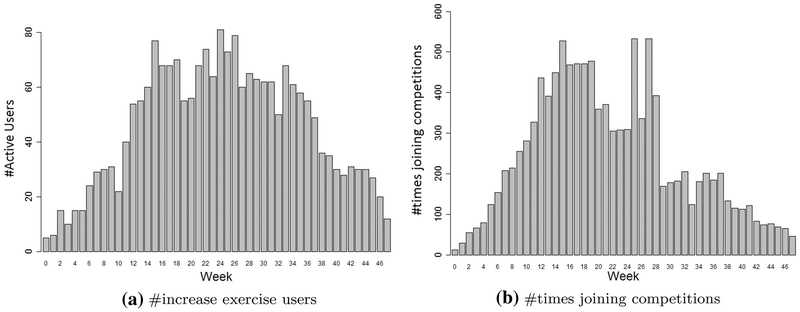
To examine the efficiency, we compare the proposed SRBM⁺ model with the competitive models in terms of human behavior prediction. Figure 5c shows the accuracy comparison over 37 weeks in our health social network. It is clear that the SRBM⁺ outperforms the other models. The accuracies of the competitive models tend to drop in the middle period of the study. All the behavior determinants and their interactions potentially become stronger, since all the users improve their activities, such as walking and running, participating in more competitions, etc. (Fig. 6) in the middle weeks. Absent or insufficient modeling of one of the determinants or of one of their interactions results in a low and unstable prediction performance. Therefore, competitive models do not well capture the social influences and environmental events. Meanwhile, the SRBM⁺ model comprehensively models all the determinants. So, the correlation between the personal attributes and the implicit social influences can be detected by the hidden variables. Thus, much information has been leveraged to predict individual behaviors. In addition, our prediction accuracy stably increases over time. That means our model well captures the growing of our health social network (Fig. 3b). Consequently, our model achieves higher prediction accuracy and a more stable performance. Overall, the SRBM⁺ model achieves the best prediction accuracy in average as 0.8941.

Fig. 6.

The distributions of users’ activities

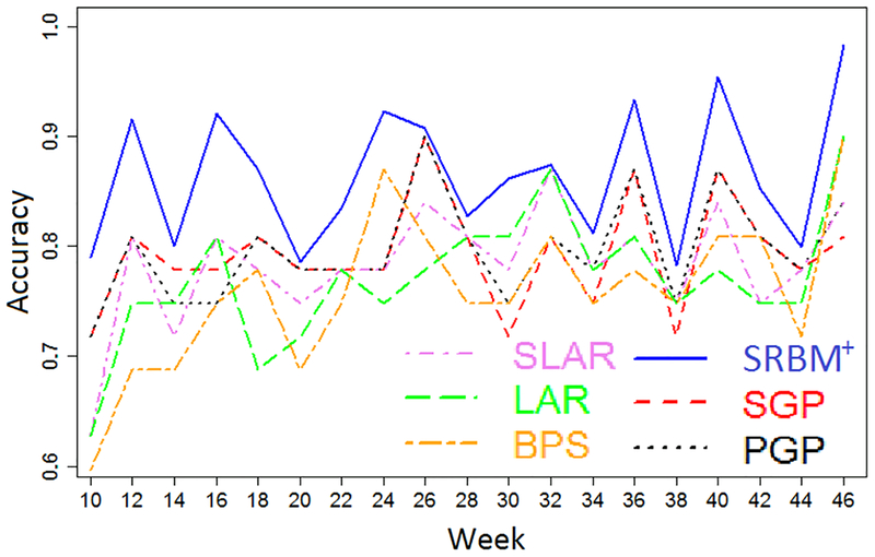
Synthetic health social network To illustrate that our model can be generally applied on different datasets, we performed further experiments on a synthetic health social network. To generate the synthetic data, we used the software Pajek² to generate graphs under the Scale-Free/Power Law Model.³ However, the vertices in the current synthetic graph do not have individual features similar to the real-word data. An appropriate solution to this problem is to apply a graph-matching algorithm to map pairwise vertices between the synthetic and real social networks. In order to do so, we first generated a graph with 254 nodes and the average node degree of 5.4 (i.e., similar to the real YesiWell data). Then, we apply PATH (Zaslavskiy et al. 2008), which is a very well known and efficient graph-matching algorithm, to find a correspondence between vertices of the synthetic network and vertices of the YesiWell network. The source code of the PATH algorithm is available in the graph-matching package GraphM.⁴ Then, we can assign all the individual features and behaviors of any real user to corresponding vertices in the synthetic network. Consequently, we have a synthetic health social network that imitates our real-world dataset. Figure 7 shows the accuracies of the conventional models and the SRBM⁺ model on the synthetic data. We can see that our model still outperforms the conventional models in terms of prediction accuracy.

Fig. 7.

Accuracies on the synthetic data

5.2. Validation of behavior determinants and explanations

5.2.1. Reliability of behavior determinants

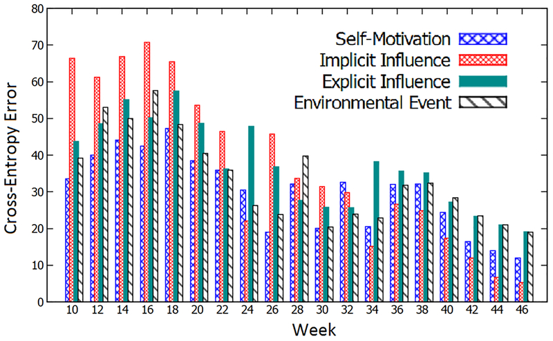
One of our main goals is to validate the reliability of the human behavior determinants that are learned in our model. We illustrate this in two comparative experiments: (1) each determinant is independently used in the SRBM⁺ model to predict behaviors of the users, and (2) each determinant will be respectively ignored in the SRBM⁺ model to predict behaviors of the users. The consistency between these comparative experiments can confirm the reliabilities of the determinants in our health social network. Figure 8 illustrates the cross-entropy errors in Eq. 14 of four determinants over 37 weeks of our data.

Fig. 8.

The cross-entropy errors of the human behavior determinants

We observed that self-motivation is more reliable than other determinants in terms of motivating users to increase their exercises in the first 10 weeks. This is because it achieves the best cross-entropy errors. Meanwhile, the implicit social influence is not effective in this period, since the users have not developed enough implicit relationships (i.e., highest cross-entropy errors). However, from the 24th week, the implicit social influence becomes one of the most reliable determinants, since it achieves lowest cross-entropy errors.

This phenomenon shows the important role of the implicit social influences in health social networks. In the meantime, the explicit social influences and environmental events behave as connecting factors, which not only influence the behaviors of users, but also associate the self-motivation and the implicit social influences together. In addition, the evolution of the determinants suggests a strong interaction among them, since there are no either absolutely reliable nor absolutely unreliable determinants.

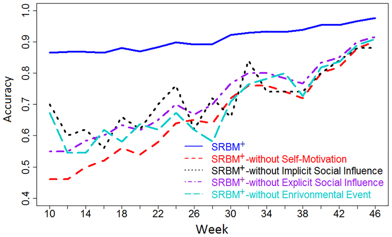
There are three meaningful observations: (1) the SRBM⁺ model enables the modeling of expressive correlations between determinants, (2) the self-motivation is especially important at the beginning, and (3) the implicit social influence will become one of the most reliable determinants, if the users have enough time to develop their relationships. These observations are strengthened by the second experiment, in which each determinant will be respectively ignored from the SRBM⁺ model to predict the behaviors of the users. Figure 9 presents the prediction accuracies of the SRBM⁺ model without each determinant respectively. It is clear that the SRBM⁺ model cannot predict behaviors of the users accurately without the self-motivation at the beginning, i.e., the prediction accuracy is notably low. This, again, confirms that the self-motivation is meaningful at the beginning. Moreover, the experiment shows the similar roles and evolution of the other determinants. The consistency between the two experiments validates the reliability of the human behavior determinants learned in our model. We have showed that the SRBM⁺ model not only achieves a significantly higher prediction accuracy compared with the conventional models, but it also offers a powerful tool to analyze the human behavior determinants. This is a breakthrough in human behavior modeling in health social networks.

Fig. 9.

Comprehensibility of the SRBM⁺

5.2.2. Human behavior explanations

Our task in this experiment focuses on answering whether the quantitative effects of human behavior determinants, denoted $\mathcal{D}=\left\{{\widehat{y}}_{t+1,\text{self}},{\widehat{y}}_{t+1,\text{im}},{\widehat{y}}_{t+1,\text{ex}},{\widehat{y}}_{t+1,\text{env}}\right\}$, offer better explanations compared with personal attributes for human behaviors.

The experiment is conducted by comparing the decision rules and trees extracted by interpretable classifiers from personal attributes and human behavior determinants, in terms of classification and prediction accuracies.

The interpretable classification models we used are 1-nearest neighbors (1-NN), decision trees (DT) (Breiman et al. 1984), node harvest (NH) (Meinshausen 2010), Ism_td (Van Assche and Blockeel 2007), ExtractedRules-PCM (E-PCM) (Fung et al. 2005), and prototype selection (PS) (Bien and Tibshirani 2011). Table 4 illustrates the accuracies of the classification on predicted behaviors, and the prediction given actual behaviors of the users.

Table 4.

Classification and prediction accuracies of interpretable classifiers in the whole dataset

Classifier		1-NN	DT	NH	Ism_td	E-PCM	PS
Personal	Classification	0.5708	0.6235	0.6835	0.6772	0.6378	0.6057
Attributes	Prediction	0.5118	0.569	0.6152	0.62	0.5984	0.553
Human Behavior	Classification	0.6639	0.836	0.8852	0.9365	0.8038	0.824
Determinants	Prediction	0.5568	0.7775	0.819	0.8682	0.7424	0.7267

In each experiment, we perform tenfold cross-validation 50 times for each algorithm, and we report the average results. It is clear that the interpretable classifiers achieve significantly better accuracies in both classification and prediction results when using human behavior determinants. This leads to an important observation: the effects of human behavior determinants which are uniquely learned by our SRBM⁺ model can be used to generate better explanations for predicted behaviors in our health social network. In addition, the Ism_td algorithm provides us the best explanations for the behaviors of users, with a very competitive prediction accuracy, i.e., 0.8682 (Table 4). Even though it achieves slightly lower accuracy than the original SRBM model, i.e., 0.8941, it still outperforms the baseline approaches (i.e., the highest accuracy is 0.7521 of the SctRBM model). The generated decision tree from the Ism_td model is made available here.⁵

6. Conclusions

This paper introduces SRBM⁺, a socialized deep learning model for human behavior prediction with explanations in health social networks. By incorporating all human behavior determinants—self-motivation, implicit and explicit social influences, and environmental events—our model predicts the future activity levels of users more accurately and more stably than conventional methods. We contribute novel techniques to deal with structural domain knowledge (i.e., ontologies) and human behavior modeling. Our experiments in a real-world health social network discover several meaningful insights: (1) user representations based on ontologies can further improve accuracies of deep learning approaches for human behavior prediction, (2) the SRBM⁺ model expressively represents all the determinants and their correlations, and (3) human behavior determinants which are learned in our model are reliable, and their quantitative effects can be used to generate better explanations compared with personal attributes for human behaviors.

Our work can be extended in several directions. First, we can leverage the knowledge-based graph to generate more descriptive explanations. Second, the approach explored in this paper is rooted on the RBM (Smolensky 1986). However, other alternatives are possible, which can be based on CNNs (Lecun et al. 1998) or Sum-Product Networks (Poon et al. 2011). We plan to explore and compare these different strategies in our future work. Third, we plan to incorporate the interpretability of our model by incorporating the explanation generating process into the optimization problem of deep learning.

References

- Bandura A (1989) Human agency in social cognitive theory. Am Psychol 44(9):1175–1184 [DOI] [PubMed] [Google Scholar]
- Barbieri N, Bonchi F, Manco F (2014) Who to follow and why: link prediction with explanations In: KDD ‘14, pp 1266–1275 [Google Scholar]
- Bien J, Tibshirani R (2011) Prototype selection for interpretable classification. Ann Appl Stat 5(4):2403–2424 [Google Scholar]
- Breiman L, Friedman JH, Olshen RA, Stone CJ (1984) Classification and regression trees. Wadsworth International Group, Wadsworth [Google Scholar]
- Christakis N (2010) The hidden influence of social networks. In: TED2010 http://www.ted.com/talks/nicholas_christakis_the_hidden_influence_of_social_networks
- Freitas AA (2014) Comprehensible classification models: a position paper. SIGKDD Explor Newslett 15(1):1–10 [Google Scholar]
- Fung G, Sandilya S, Rao RB (2005) Rule extraction from linear support vector machines In: KDD’05, pp 32–40 [Google Scholar]
- Kawale J, Pal A, Srivastava J (2009) Churn prediction in mmorpgs: a social influence based approach In: CSE’09, pp 423–428 [Google Scholar]
- Kil D, Shin F, Piniewski B, Hahn J, Chan K (2012) Impacts of social health data on predicting weight loss and engagement In: O’Reilly StrataRx Conference [Google Scholar]
- Lecun Y, Bottou L, Bengio Y, Haffner P (1998) Gradient-based learning applied to document recognition. Proc IEEE 86(11):2278–2324 [Google Scholar]
- Lerman K, Intagorn S, Kang JK, Ghosh R (2012) Using proximity to predict activity in social networks In: WWW’12 Companion, pp 555–556 [Google Scholar]
- Li X, Du N, Li H, Li K, Gao J, Zhang A (2014) A deep learning approach to link prediction in dynamic networks In: SDM’14, pp 289–297 [Google Scholar]
- Marshall A, Eakin E, Leslie E, Owen N (2005) Exploring the feasibility and acceptability of using internet technology to promote physical activity within a defined community. Health Promot J Aust 2005(16):82–84 [DOI] [PubMed] [Google Scholar]
- Meinshausen N (2010) Node harvest. Ann Appl Stat 4(4):2049–2072 [Google Scholar]
- Page L, Brin S, Motwani R, Winograd T (1999) The pagerank citation ranking: bringing order to the web. Technical Report 1999–66, Stanford InfoLab [Google Scholar]
- Pate R, Pratt M, Blair S et al. (1995) Physical activity and public health: a recommendation from the centers for disease control and prevention and the american college of sports medicine. JAMA 273(5):402–407 [DOI] [PubMed] [Google Scholar]
- Phan N, Dou D, Piniewski B, Kil D (2015) Social restricted boltzmann machine: Human behavior prediction in health social networks In: ASONAM’15, pp 424–431 [DOI] [PMC free article] [PubMed] [Google Scholar]
- Phan N, Dou D, Xiao X, Piniewski B, Kil D (2014) Analysis of physical activity propagation in a health social network In: CIKM’14, pp 1329–1338 [Google Scholar]
- Poon H, Domingos P (2011) Sum-product networks: a new deep architecture In: UAI’11, pp 337–346 [Google Scholar]
- Ryan RM, Deci EL (2000) Intrinsic and extrinsic motivations: classic definitions and new directions. Contemp Educ Psychol 25(1):54–67 [DOI] [PubMed] [Google Scholar]
- Shen Y, Jin R, Dou D, Chowdhury N, Sun J, Piniewski B, Kil D (2012) Socialized gaussian process model for human behavior prediction in a health social network In: ICDM’12, pp 1110–1115 [DOI] [PMC free article] [PubMed] [Google Scholar]
- Siegel E (2013) Predictive analytics—the power to predict who will click, buy, lie or die. Wiley, Hoboken [Google Scholar]
- Smolensky P (1986) Information processing in dynamical systems: foundations of harmony theory. Parallel Distrib Process Explor Microstruct Cognit 1:194–281 [Google Scholar]
- Taylor G, Hinton G, Roweis S (2006) Modeling human motion using binary latent variables In: NIPS’06, pp 1345–1352 [Google Scholar]
- Ustun B, Rudin C (2014) Methods and models for interpretable linear classification. ArXiv e-prints [Google Scholar]
- Van Assche A, Blockeel H (2007) Seeing the forest through the trees: learning a comprehensible model from an ensemble In: ECML’07, vol 4701, pp 418–429 [Google Scholar]
- Viswanath B, Mislove A, Cha M, Gummadi K (2009) On the evolution of user interaction in facebook In: WOSN’09, pp 37–42 [Google Scholar]
- Yang J, Wei X, Ackerman M, Adamic L (2010) Activity lifespan: An analysis of user survival patterns in online knowledge sharing communities In: ICWSM’10 [Google Scholar]
- Zaslavskiy M, Bach F, Vert JP (2008) A path following algorithm for graph matching. IEEE Trans Pattern Anal Mach Intell 5099:329–337 [DOI] [PubMed] [Google Scholar]
- Zhu Y, Zhong E, Pan S, Wang X, Zhou M, Yang Q (2013) Predicting user activity level in social networks In: CIKM’13, pp 159–168 [Google Scholar]