Two-Dimensional Frequency-Swept Pulse with Resilience to Both B₁ and B₀ Inhomogeneity

Abstract

Applications of multidimensional spatially-selective pulses are sometimes limited by their long pulse durations resulting from the need to execute a modulated gradient waveform in concert with RF transmission. Here, we introduce a method to design two-dimensional selective adiabatic pulses using a Cartesian k-space trajectory. The full pulse can be sampled using various undersampled segments to create a multidimensional pulse resilient to large off-resonances. Moreover, the pulse can be designed to be resilient to B₁⁺ inhomogeneity. Experimental demonstrations of fully segmented and single-shot k-space sampling patterns are presented.

Graphical abstract

INTRODUCTION:

Two- (2D) and three-dimensional (3D) MRI methods usually employ radiofrequency (RF) pulses that are spatially selective in one direction only. Following RF excitation, phase encoding in one or more directions is then used to spatially encode the ensuing signal. Since this is a Fourier encoding strategy, Nyquist’s criterion must be met, which necessitates using a field-of-view (FOV) at least as large as the object in all directions. When a high resolution is desired in the phase-encoded direction(s), this condition can lead to lengthy acquisition times. To reduce the acquisition time, a RF pulse that is selective in more than one spatial dimension can be used to delineate a smaller FOV in one or more of the phase-encoded dimensions.

As first described by Pauly et al. [1], multidimensional small tip angle pulses may be described by a parameterized trajectory through k-space, where the trajectory is determined by the linear field gradients used during the pulse. That work was then extended to large tip angle pulses by Pauly et al. [2], where it was shown that a large tip angle could be achieved if the pulse could be decomposed into several inherently refocused, small tip angle pulses. Here, inherently refocused is synonymous with returning to $\overrightarrow{k}=0$ in pulse k-space. All these 2D pulses were performed in a single shot; in other words, the entirety of k-space was sampled for the pulse in one excitation. A similar approach by Conolly et al. [3] repeatedly plays out sine pulses during an oscillating echo-planar type of gradient train. The peak amplitude and initial phase of each sine pulse are modulated according to those of a hyperbolic secant pulse [4] to produce a 2D adiabatic pulse. For this 2D pulse and others similar to it, the large number of pulses necessary to fully sample the 2D k-space of the pulse can lead to prohibitively long pulse duration.

In the 2D pulses of Conolly et al. [3], the bandwidth of the pulse in the direction of the oscillating gradient can be increased by using a frequency-modulated (FM) pulse in place of the amplitude-modulated sine pulses. This was the approach taken by Dumez et al. [5], whereby chirp pulses were used in both dimensions. The pulse design in that work was described in physical space, not in k-space, and equations describing the pulse design were not given.

Here, we describe a 2D RF pulse which is a hyperbolic secant pulse in both dimensions in k-space. We use an echo-planar imaging (EPI) [6] gradient train during the excitation, and increase the low bandwidth achieved in the slow dimension of the pulses used in previous works. Specifically, we undersample different segments of the pulse to decrease the length of each pulse segment, thus increasing the bandwidth for a fixed time-bandwidth product, R.

Hereafter, the direction of the oscillating gradient will be referred to as the fast-selected dimension, while the direction of the blipped gradient will be referred to as the slow-selected dimension. This nomenclature is due to the relative time needed for spatial selection in each dimension. As was done by Jang et al. [7], B₁⁺ inhomogeneity will be addressed by scaling the time-dependent RF amplitude based on a B₁⁺ map and having knowledge of the spatiotemporal vertex produced by the 2D FM pulse.

THEORY:

Two-dimensional Cartesian excitation:

Denoting a normalized k-space vector by κ_f,s∈[−1,1] in the fast and slow dimensions, respectively, the amplitude- and phase-modulated functions of the RF pulse, as defined in terms of the pulse’s k-space trajectory, are

$${\omega }_1={\omega }_{1,\mathit{max}}\mathrm{sech}\left(\beta {\kappa }_f(t)\right)\mathrm{sech}(\beta {\kappa }_s(t))$$ 1

$${\varphi }_{\mathit{RF}}=A_f\log \left(\mathit{cos}h\left(\beta {\kappa }_f(t)\right)\right)\pm A_s\log \left(\mathit{cos}h\left(\beta {\kappa }_s(t)\right)\right)$$ 2

In these equations, β determines where these functions are truncated, and in the present work, its value was determined according to sech(β) = 0.01 (i.e., the amplitude-modulated function truncates at 1% of maximum). In Eq 2, choosing the positive sign leads to a parabolic phase over the object, while a negative sign yields a hyperbolic phase profile. For the remainder of this work, the negative sign will be used. Additionally, κ_f,s are normalized by $({\omega }_1^{\mathit{max}}=\gamma B_1^{\mathit{max}})$, which is Eq [7] of Ref [1]. Denoting the time-bandwidth product of the pulse in the fast and slow dimensions as R_f and R_s respectively, the coefficients A_f,s are defined by $A_{f,s}=\frac{\pi R_{f,s}}{2\beta }$. The formulae given yield a rectangular excitation profile, although the same trajectory can be used with the k-space weighting as described by Jang et al. [7] to obtain a circular excitation profile. In the latter case, the single-shot Cartesian trajectory also yields an adiabatic pulse. Profile thickness is given in both dimensions of the current pulse as

$$\Delta x_{f,s}=\frac{R_{f,s}}{2k_{\{f,s\},\mathit{max}}}$$ 3

where f and s denote the fast and slow dimensions, respectively. For B₁ compensation, the instantaneous vertex position is given by

$$x_{f,s}(t)=\frac{\Delta x_{f,s}}{2}{\kappa }_{f,s}(t)$$ 4

Further below it will be shown how Eq [4] can be used to modify the pulse to produce a uniform flip angle with a spatially-varying RF field, B₁⁺. While the 2D spatial selection can be performed in any orientation, the fast and slow spatially-selected dimensions will herein generally be referred to as X and Y, respectively.

Segmentation:

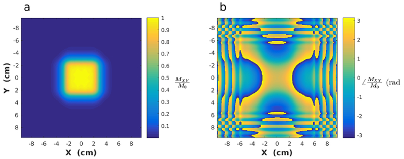
As mentioned in the Introduction, the bandwidth in the fast-selected dimension can be further increased by replacing the sinc pulses in the 2D pulse by Conolly et al. [3] with frequency-swept pulses. The 2D frequency-swept pulses in this work are based on the original hyperbolic secant pulse, HS1 [4], but other frequency-swept pulses can also be used, including higher order HSn pulses [8] or a chirp pulse [9], as was done by Dumez et al. [5]. The k-space representation of this pulse and its Bloch simulated excitation profile are shown in Fig. 1. The bandwidth in the slow-selected dimension can be increased by only sampling segments of the fully sampled 2D pulse with each excitation, as shown in Fig. 2. This decreases the pulse length while maintaining R, such that the bandwidth in the slow dimension increases in inverse proportion to the pulse length reduction. However, to retain the desired 2D excitation profile, a full image readout must be acquired for each pulse segment. Depending on the specific sequence used, this might necessitate a complex tradeoff between minimum scan time and pulse bandwidth, since as the pulse is shortened, the minimum possible repetition time TR decreases. For a fixed TR, the total acquisition time scales linearly with the number of pulse segments used. At the end of all acquisitions, the data are summed over all segments in either k-space or image space with the appropriate weights.

Figure 1:

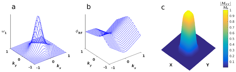
k-space description of the 2D pulse. a) The RF amplitude as a function of k-space. b) The RF phase as a function of k-space. c) The transverse magnetization (M_xy) profile produced by this pulse.

Figure 2:

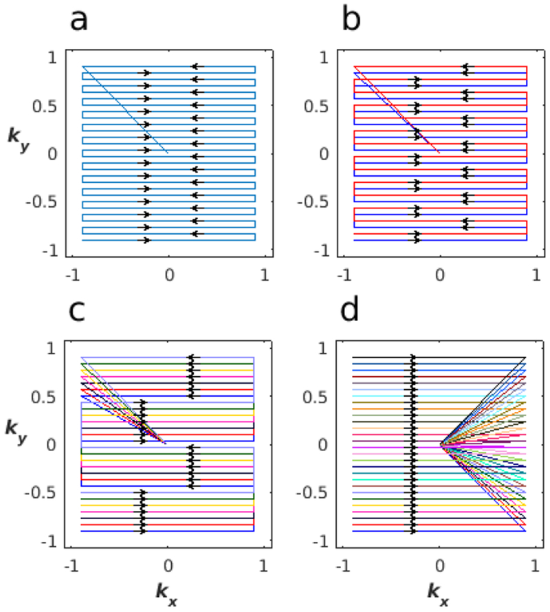
Example k-space trajectories for a 2D RF pulse. a) A single segment coverage of k-space. b) Covering k-space in 2 segments, with each segment sampling 14 equidistant lines of k-space. c) 7-segment trajectory, with each segment sampling 4 equidistant lines of k-space. d) Fully segmented trajectory, sampling only 1 line of k-space with each segment. Another option for segmented pulses is to alternate the initial direction of the k-space trajectory between segments, which gives different off-resonant behavior. Trajectories do not need to be interleaved as shown. Segmented trajectories which sample k-space sequentially and do not overlap are also possible. Colors were chosen using [23].

Using a 2D pulse permits increased spatial resolution in a fixed imaging time by decreasing the FOV in the phase-encoded dimensions of an experiment. By segmenting the pulse with a fixed TR, the acquisition time increases multiplicatively with the number of segments. Thus, to avoid increasing imaging time, the number of segments used must not exceed the acceleration gained by shrinking the FOV. If we assume that phase encoding is performed in the zoomed spatial dimensions, then the number of segments N_seg should ideally satisfy

$${\mathrm{N}}_{\mathrm{seg}}\le \frac{{\mathrm{PE}}_{1,\text{full}}}{{\mathrm{PE}}_{1,\text{zoomed}}}\frac{{\mathrm{PE}}_{2,\text{full}}}{{\mathrm{PE}}_{2,\text{zoomed}}}$$ 5

to not increase the imaging time, where PE_i,full and PE_i,zoomed denote the number of phase encoded steps in a given dimension (i) in the full and zoomed FOV, respectively. This assumes equal resolution between zoomed and full FOV scans.

To sample each segment correctly in pulse k-space, care must be taken to ensure each segment has the same k-space center defined. Since the k-space trajectory is defined by the integral of the remaining gradient, there must be a variable area gradient lobe at the end of each segment in the slow-selected dimension. If these refocusing lobes are not the correct magnitude and polarity, different segments may amount to sampling the pulse multiple times along the same line(s) of k-space. Hence, the trajectory of a given segment depends crucially on the refocusing gradient, and the sampling weight depends on the RF amplitude and phase. Thus, even though each segment can use the same gradient waveform during RF transmission, its exact trajectory in k-space is determined by the gradient refocusing lobe that follows the RF pulse(s) of a given segment.

Obtaining consistent contrast:

As a consequence of the amplitude modulation in the 2D HS1 pulse, each pulse segment produces a different flip angle. As a result, under the commonly used acquisition condition TR ≪ T₁, the different pulse segments produce variable T₁-weighting of the image data. This can be remedied by rescaling the power of each pulse segment to achieve a constant flip angle for all segments. However, during the summation over all segments used, perfect signal cancellation outside the desired selected region does not occur. This issue is readily solved by reweighting the reconstruction of each segment with a weight equal to the original flip angle of the segment. For a fully segmented pulse in which one line of k-space is sampled per segment, this procedure then amounts to reweighting each reconstruction according to a HS1 pulse defined by the number of segments used. For a partially segmented pulse, the data for each segment is scaled in post-processing by the integral of the respective pulse segment. The weights are given by

$$C_i=\mid {\int }_0^T{\omega }_{1,i}(t)\mathit{exp}\left(-j{\Phi }_{\mathit{RF},i}(t)\right)\mathit{dt}\mid$$ 6

where the subscript i denotes segment number and j the square root of −1.

When undersampling a pulse, the sidebands in the slow dimension move closer to the baseband as the number of segments increases. The signals from these sidebands cancel only after summing the acquired data. When a pulse segment is undersampled beyond the Nyquist limit, the sidebands and baseband overlap, and this leads to a non-uniform flip angle per segment. Thus, in this case, despite maintaining the proper excitation region after summation, it is not possible to obtain a consistent flip angle across the entire excitation region for each segment. However, when using a fully segmented pulse, such spatial variation of the flip angle in the slow dimension does not occur for any segment. In this limiting case, there is again uniform T1 contrast within the desired profile.

While rescaling the pulse amplitude to achieve the same flip angle for each segment gives equal SNR for each readout, rescaling the data in post-processing before summation yields a suboptimal SNR. The exact SNR can be calculated using Eq. 2 of [10], wherein the SNR as a fraction of the maximum possible for N segments is

$$\mathrm{SNR}=\frac{\sum _{\mathrm{i}=1}^N\mid C_i\mid }{\sqrt{N\sum _{\mathrm{i}=1}^N{\mid C_i\mid }^2}}$$ 7

where the C_i are the coefficients used to scale the data in post-processing.

B₁⁺ Compensation:

Because the pulse is phase modulated in two spatial domains, 2D spatiotemporal excitation takes place during the pulse in a manner that is dictated by the resulting (rasterized) trajectory of a hyperbolic phase function in space. By assuming excitation at a given moment is localized to the vertex of this hyperbolic phase function, the 2D pulse can be modified to achieve uniform flip angle despite the existence of significant B₁⁺ inhomogeneity. The process begins by obtaining a unitless B₁⁺ map (denoted by B_1,c⁺) that is normalized to 1 at its maximum. Then the RF waveform can be recalculated as

$${\omega }_{1,c}(t)=\frac{{\omega }_1(t)}{B_{1,c}^{+}\left(x_f(t),x_s(t)\right)}$$ 8

where x_f and x_s describe the vertex position in the fast and slow dimensions respectively. In areas where the B₁⁺ map is not well defined, the original pulse value may be used.

Simulations:

Adiabaticity and Off-Resonance Effects:

The simulated pulse consisted of 28 lines of k-space describing the pulse in the slow dimension. Additionally, the R value in both directions of the pulse was set to 9 and the slab thickness set at 5 cm. Each subpulse element, which samples one line of pulse k-space, was 700 μs. The duration of the gradient blips in the slow dimension were 120 μs with a half-sinusoid shape. Taken together with the number of lines of k-space, these parameters fully define the 2D pulse according to Eqs [1–3]. An example MATLAB script for creating a segmented 2D HS1 pulse is found in [11]. In the following simulations, relaxation effects have been ignored.

As shown in Fig. 3., the 2D HS1 pulse can be driven adiabatically when sampled on a Cartesian k-space trajectory, in contrast to the 2D spiral trajectory described in [7]. When driven sub-adiabatically (Figs. 3a and 3b), the 2D excitation profile remains square and unchanged even when altering the excitation flip angle. When driven adiabatically, the cross section through the fast dimension (Fig. 3c) becomes wider than that through the slow dimension (Fig. 3d) as the peak RF amplitude $({\omega }_1^{\mathit{max}}=\gamma B_1^{\mathit{max}})$ increases. This happens because the transition regions in the profile of each subpulse undergo adiabatic inversion in the process of executing the full 2D pulse.

Figure 3:

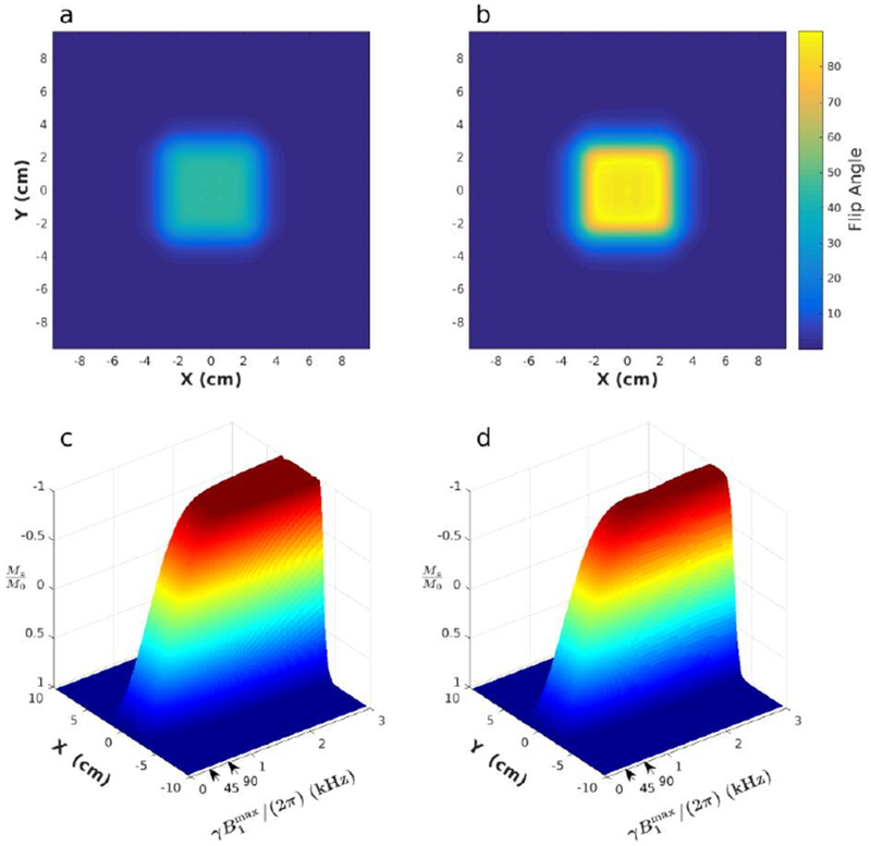
Demonstration of the non-adiabatic and adiabatic regimes of the single shot 2D pulse. a) Transverse magnetization when applying the single-shot pulse for a 45° excitation. b) Transverse magnetization when applying the single-shot pulse for a 90° excitation. Notice the profile width is unchanged in both spatial dimensions. c) Surface plot showing the normalized longitudinal magnetization along the fast dimension as a function of B₁^max when traversing all of k-space in a single shot. When the pulse begins operating adiabatically, the transition regions begin to invert, increasing the slab width in the fast dimension. d) Surface plot showing the longitudinal magnetization along the slow dimension as a function of B_L^max when traversing all of k-space in a single-shot. B₁^max denotes the peak B₁ used in t he pulee. Arrows in (c) and (d) indicate the RF amplitude settings used to obtain the 4° and 90° flip angles for (a) and (b).

The Bloch simulated magnitude and phase of the excitation profile are shown in Fig. 4. Similar cross sections showing the excitation profile through the fast and slow dimensions for various offset frequencies are given in Fig. 5. In the ideal case, there should be no dependence of the excitation profile on offset frequency, but Bloch simulations reveal the inability of the single-shot pulse to maintain a consistent profile in the presence of large frequency offsets in either the fast or slow dimensions. Despite the large bandwidth in the fast dimension, frequency offsets prevent spin isochromats from returning through $\overrightarrow{k}=0$ with each sweep, marring the profile in that direction. In the slow dimension, constant frequency offsets cause translations in physical space of the excitation profile. As the number of pulse segments is increased, the fast dimension noticeably improves in quality. In the slow dimension, it can be observed that the unwanted transverse magnetization away from the desired excitation region has diminished in amplitude relative to the single shot case, although this is not as apparent as in the fast dimension. For the fully segmented pulse, the selected region exhibits only translation in physical space as a function of the frequency offset, while the slow dimension exhibits complete independence from constant frequency offsets.

Figure 4:

Excitation profile of the 2D pulse for any number of segments. a) Magnitude of the normalized transverse magnetization profile at the end of the pulse for any number of segments, provided they are properly weighted prior to summing. b) Phase of the transverse magnetization profile (radians).

Figure 5:

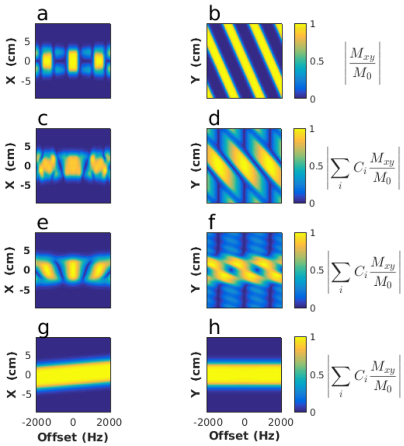
Excitation profile behavior for various frequency offsets and number of pulse Segments. a) Normalized transverse magnetization profile along the fast dimension versus a constant frequency offset when traversing all of k-space in a single shot. Note the rapid degradation of the profile with small offsets. b) The profile along the slow spatially-selected dimension versus a constant offset. Sidebands are intense and near the center band. c) With 2 segments defining the pulse, the profile in the fast dimension versus a constant offset is beginning to improve, while in d) the sidebands in the slow dimension are still prominent. e) Using 7 segments to define the pulse, the fast dimension has improved further. f) With 7 segments, the sidebands in the slow dimension are noticeably diminished in amplitude. g) With the fully segmented pulse, the profile simply shifts in physical space with a constant offset in the fast dimension, while in h), there is no dependence on constant offsets in the slow dimension. Rows 1-4 use the respective k-space trajectories shown in Figs. 2a - 2d. The complex transverse magnetization is given by M_xy = M_x + j M_y and the coefficients C_i are defined in the text as equation 6.

Such a dramatic difference between the fully segmented pulse and any of the partially segmented pulses can be understood as follows. Ideally, the transverse magnetization does not freely evolve between different sampling times of k_fast = 0. If the time between sampling k_fast = 0 for any number of segments is given by τ the transverse magnetization evolves an amount

$$\Phi =\delta \tau$$ 9

between subpulses, where δ is a constant frequency offset. In the fully segmented pulse, these phases are identical for all pulse segments, whereby their effects are cancelled perfectly. For any other number of segments, the phase offset results in additional phase offsets in k-space. This gives an imperfect cancellation of transverse magnetization for off-resonant spins.

MATERIALS AND METHODS:

All experiments were performed with a Varian DirectDrive console (Agilent Technologies, Santa Clara, CA) interfaced with a 4T, 90-cm magnet (Oxford Magnet Technology, Oxfordshire, UK) and a clinical gradient system (model SC72, Siemens, Erlandgen, Germany). The maximum slew rate available on this gradient system is 100 mT/m/ms. Experimental verifications of the fully segmented and single-shot imaging sequences were performed using the pulse parameters described in the simulations section. A protocol approved by our institution’s IRB was followed for human brain imaging of healthy volunteers after written, informed consent was obtained.

Gradient pre-emphasis for the fast gradient direction was performed using the gradient impulse response function (GIRF) [12], which is measured by using triangular gradient waveforms of varying width and amplitude on each gradient channel to fully sample the GIRF in the frequency domain. Gradient waveforms were measured following a protocol similar to Stich et al. [13], where 12 triangular waveforms were employed with amplitudes distributed linearly from 0.3125 G/cm to 3.75 G/cm. The slew rate of each waveform was set to 0.9 times the maximum possible to minimize waveform errors from the gradient amplifiers. The offset slice method [14] was used to measure the waveforms. In this method, a single 1-mm thick slice was offset 1.5 cm from isocenter for each gradient channel. The readout bandwidth was 50 kHz and the total readout time was 17 ms to obtain a spectral resolution of 58.82 Hz. Thirty averages were used with TR = 6 s and TE = 13.83 ms. Gradient pre-emphasis was necessary to prevent Nyquist ghosting of the excitation profile which results when there is a mismatch in sampling of k = 0 between the positive and negative gradient polarities.

Due to the longer minimum T_R necessary for the single-shot excitation, T₂*-weighted imaging was performed with this sequence, using a flip angle of 15°, TR/TE = 41.5 ms/25 ms with one average. The total single-shot pulse length was 23.704 ms. The receiver bandwidth was set at 100 kHz. Using the same total acquisition time, a full brain image was acquired at 1.6 mm isotropic resolution with a FOV = 192 × 192 × 192 mm³. Identical sequence settings were used with the single-shot pulse to demonstrate spatial selectivity, followed by a sequence which zoomed on the selected region. The isotropic resolution of this zoomed experiment was 800 μm with a FOV = 192 × 96 × 96 mm³ with the same total imaging time of 7.6 minutes.

A demonstration of B₁⁺ compensation was performed using the single-shot sequence on a uniform agar phantom and a quadrature surface coil for excitation and reception. The B₁⁺ profile was measured using the double angle method (DAM) [15], while the B₁⁻ map was measured using an adiabatic half passage excitation followed by two adiabatic full passages for refocusing. Each of these pulses was operated with sufficient RF power to be in the adiabatic regime. Reconstructed images were divided by the B₁⁻ map where there was sufficient signal to divide by. This level was taken as 10% of the maximum image intensity in the B₁>⁻ map.

For the fully segmented sequence, a 3D T₁-weighted GRE sequence was used with TR/TE = 6.09 ms/2.76 ms, flip angle = 10.4°, and receiver bandwidth = 100 kHz. Isotropic resolution of 1.5 mm³ was used, with a FOV = 192 × 96 × 96 mm³. To demonstrate robustness to B₀ inhomogeneity, an additional experiment was performed in which one linear gradient was held fixed throughout the duration of the imaging sequence. A B₀ map was measured for a single slice, which demonstrated the constant gradient was approximately 16.66 kHz over 19 cm in the slow-selected direction of the pulse.

RESULTS:

The surface coil experiment provided an extreme case of B₁ inhomogeneity for demonstrating B₁⁺ compensation. The relative improvement in the excitation profile can be seen in Fig. 6, where the results of the compensated and uncompensated pulses are shown after dividing by the B₁⁻ map. The lower flip angle in the B₁⁺ compensated image is due to a lower average RF power in the compensated pulse when using the same peak power.

Figure 6:

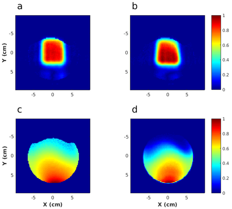
Experimental demonstration of the B₁⁺ compensation method described in the text. a) Excitation profile obtained using the B₁⁺-compensated pulse. b) Excitation profile obtained using the original pulse. Both a) and b) have been divided by the receive coil sensitivity shown in (d), which was measured using the sequence described in the text. c) Transmit (B₁⁺) map measured using the double angle method.

Selected cross sections from 3D brain images obtained with the single shot and fully segmented pulses are shown in Figs. 7 and 8, respectively. The single-shot pulse was used for excitation in a T₂*-weighted sequence while the fully segmented pulse was used in a T₁-weighted sequence. The fully segmented version yields the most well-defined excitation profile, since it is essentially immune to off-resonance effects. This is clearly seen in the images collected with a constant gradient on during the sequence, where the excited profile is nearly identical to that obtained in a homogeneous field.

Figure 7:

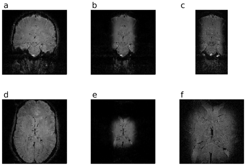
In vivo brain images obtained with a 3D T₂*-weighted GRE imaging sequence, using TR = 41.5 ms, TE = 25 ms, and flip angle = 15°. a - c) Coronal cross sections. d - f) Axial cross sections. a,d) FOV = 192 × 192 mm², isotropic resolution of 1.6 mm², with a non-selective excitation. b,e) FOV = 192 × 192 mm², isotropic resolution of 1.6 mm², with single-shot 2D HS1 excitation. c,f) FOV = 192 × 96 mm², isotropic resolution of 0.8 mm², with single-shot 2D HS1 excitation.

Figure 8:

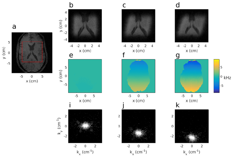
Brain images obtained with a T₁-weighted 3D GRE acquisition. Sequence parameters were TR = 6.09 ms, TE = 2.76 ms, and flip angle = 10.4°. a) A single plane is shown from this dataset. The red box depicts the zoomed FOV used for (b – d). The in-plane resolution of this cross section is 1 mm² and FOV = 192 × 192 mm², while the through-plane resolution was 1 mm. b) The same sequence parameters as (a) except a fully segmented pulse was used for excitation. The in-plane resolution of this cross section is 1.5 mm² and FOV = 96 × 96 mm², while the through-plane resolution was 1.5 mm. The B₀ map for this case is shown in e). c) The same as (b), except the acquisition was performed in the presence of a constant field inhomogeneity created by turning on a gradient in the y-direction and leaving it on for the duration of the sequence. The measured B₀ for this dataset is given in f). In d), the gradient was set even higher, creating a frequency variation of approximately 16.66 kHz across the brain in the slow dimension of the pulse. The corresponding B₀ map is given in g). Note that all B₀ maps are shown on the same scale to demonstrate the magnitude of the inhomogeneity. This obscures the small fluctuations in (e) as they are significantly smaller than those in (f) and (g). In both (c) and (d). the static gradient in the slow dimension causes a change in orientation of the gradient during excitation, resulting in a tilted profile, i) – k) The log-scale Fourier domain of the data shown in (b – d), respectively. Note how there is no additional signal loss from the constant gradient, but only a shift in k-space.

DISCUSSION & CONCLUSIONS:

Single-shot multidimensional pulses require long pulse lengths, which decreases their bandwidth. Herein, we have shown how undersampling a multidimensional pulse by segmenting it and adding the resultant segments together after data collection permits shorter pulses, in turn leading to higher bandwidths. To the best of our knowledge, this work describes the first experimental implementation of a frequency-swept pulse in a multi-shot (segmented) form, whereas only amplitude-modulated pulses have been implemented in segments previously ([16]–[18]). The method of segmenting a 2D EPI excitation trajectory was first proposed by Panych et al. [16], while the first segmented pulses were interleaved spirals [17]. Previously, segmented 3D pulses have been shown to be useful in 2D MRI for slice selection and B₀ compensation [18]. In the segmentation method of Panych et al. [16], a 2D excitation profile was defined using a segmented EPI k-space trajectory with B₁ amplitudes given by the Fourier transform of the desired excitation shape. To obtain consistent T₁ contrast, an equal flip angle was assumed to be produced by every pulse segment without rescaling the RF power used for transmitting each segment. This condition cannot be satisfied when using shaped pulses. That work also did not focus on the use of a segmented 2D EPI trajectory to increase the pulse bandwidth, as done herein. Finally, previously described segmented pulses ([16]—[18]) do not permit the herein described method of B₁⁺ compensation since they are not FM pulses.

Although the imaging experiments presented demonstrate only the single-shot and fully segmented cases, it should be noted that any number of segments can be used to fully sample the pulse. However, use of an integer divisor of the number of lines of k-space is recommended, so that the number of subpulses, the subpulse length, and the total pulse length are all equal between segments. If this condition is not met, care must be taken to ensure TR and TE are maintained between segment acquisitions. It should be noted that diffusion effects may differ between segments outside of this recommended pulse design regime. Also, while here the pulse shapes along both directions were HS1 pulses, this need not be the case. For example, a sine pulse could be used for modulation in the slow dimension.

Although not demonstrated in the experiments, this 2D HS1 pulse which samples k-space on a Cartesian grid can be used to invert magnetization in an adiabatic manner, provided B₁^max is above the threshold needed to satisfy the adiabatic condition. Here, B₁^max denotes the peak B₁ of the pulse. Conversely, the previously described 2D HS1 pulse of Jang et al. [7] which utilizes a spiral k-space trajectory cannot achieve adiabaticity, regardless of the B₁^max value. A juxtaposition of the Cartesian k-space trajectory described herein with the spiral trajectory of Jang et al. [7] helps to elucidate how the different trajectories through the pulse’s k-space determine the magnetization profile with respect to frequency offset for a specific k-space weighting function, such as the 2D HS1 pulse. For the Cartesian sampling scheme, the pulse behaves adiabatically using the single-shot trajectory, due to the adiabatic frequency sweep in the slow dimension. The subpulses are frequency swept, but by themselves are not necessarily functioning adiabatically. Unfortunately, when the 2D k-space trajectory is segmented, the pulse cannot function adiabatically because the segmentation process creates discontinuities in the frequency sweep. For this reason, a segmented 2D HS1 pulse is not useful for adiabatic inversion, while the single-shot pulse is practical for such purposes.

When driven sub-adiabatically (e.g. for excitation), there exists a unique method to compensate for B₁⁺ inhomogeneity. This method is that used by Jang et al. [7], where the pulse is compensated along the trajectory of a moving vertex in physical space. Note again that this method of compensation cannot be achieved with amplitude-modulated 2D pulses since a vertex trajectory cannot be created. It is unique to multidimensional FM pulses.

Upon inspection of the results of the fully segmented pulse (see Fig. 8), no noticeable loss of signal can be seen despite the large increase in B₀ inhomogeneity imposed by the constant gradient field. The inhomogeneity merely shifts the position of the acquired data in k-space and produces a tilt in the excitation profile. Provided the acquisition k-space shift does not preclude a large amount of the signal energy from being sampled, no significant signal loss occurs. This condition is met provided the shift is smaller than k_max, the largest acquisition k-value sampled. Hence, for a given resolution Δx and echo time TE, the following must be satisfied

$$k_{\mathit{shift}}=\gamma G_{\Delta }{T}_E<k_{\max }=\frac{1}{2\Delta x}$$ 10

where G_Δ is a constant linear field inhomogeneity. This equation should hold true for non-linear inhomogeneous fields as well. In that case, G_Δ is the local field gradient and G_Δ is a function of x (i.e G_Δ(x)). That is, the k-space center position varies depending on the location of each isochromat in space.

By virtue of its hyperbolic phase profile, this pulse has potential applications in xSPEN MRI [19], [20]. In that method, a hyperbolic phase profile permits an acceleration of data acquisition by utilizing the correlation between k-space and image space when a hyperbolic or parabolic phase profile is present. These correlations exist due to the localization of signals originating from the vertex of the phase profile. Hence, the k-space signal appears as a transposed, low-resolution version of the resulting image. This approach was not taken in the present work since the gradient slew rate limitations precluded the use of high time-bandwidth products while maintaining a reasonable pulse length.

In summary, the combination of the features discussed thus far makes 2D frequency-swept pulses an attractive candidate when resilience to large B₀ and B₁⁺ field inhomogeneities is needed. To increase the bandwidth further in the future, parallel transmission techniques [21], [22] might be employed to further decrease the pulse length and drive up the bandwidth.

Highlights.

• 2D frequency swept pulses can be modified to compensate for B₁ inhomogeneity.

• In a single-shot, Cartesian sampling of a 2D HS1 yields an adiabatic pulse.

• Segmenting pulse k-space in multiple undersampled segments increases their bandwidth by shortening pulse length.

• Fully segmenting the pulse’s k-space yields almost complete immunity to B₀ inhomogeneity.

REFERENCES

- [1].Pauly J, Nishimura D, and Macovski A, “A k-space analysis of small-tip-angle excitation,” J Magn Resort, vol. 81, pp. 43–56, 1989. [DOI] [PubMed] [Google Scholar]
- [2].Pauly J, Nishimura D, and Macovski A, “A linear class of large-tip-angle selective excitation pulses,” J. Magn. Reson, vol. 82, no. 3, pp. 571–587, 1989. [Google Scholar]
- [3].Conolly S, Pauly J, Nishimura D, and Macovski A, “Two-dimensional selective adiabatic pulses,” Magn. Reson. Med, vol. 24, no. 2, pp. 302–313, 1992. [DOI] [PubMed] [Google Scholar]
- [4].Silver M, Joseph R, and Hoult D, “Highly selective and π pulse generation,” J. Magn. Reson, vol. 59, no. 2, pp. 347–351, 1984. [Google Scholar]
- [5].Dumez JN and Frydman L, “Multidimensional excitation pulses based on spatiotemporal encoding concepts,” J. Magn. Reson, 2013. [DOI] [PubMed] [Google Scholar]
- [6].Stehling MK, Turner R, and Mansfield P, “Echo-Planar Imaging: Magnetic Resonance Imaging in a Fraction of a Second,’ Science (80-, ), vol. 254, no. 5028, pp. 43–50, 1991. [DOI] [PubMed] [Google Scholar]
- [7].Jang A, Kobayashi N, Moeller S, Vaughan JT, Zhang J, and Garwood M, “2D Pulses using spatially dependent frequency sweeping,” Magn. Reson. Med, vol. 76, no. 5, pp. 1364–1374, 2016. [DOI] [PMC free article] [PubMed] [Google Scholar]
- [8].Tannús A and Garwood M, “Adiabatic pulses,” NMR Biomed, vol. 10, no. 8, pp. 423–434, 1997. [DOI] [PubMed] [Google Scholar]
- [9].“Dunant JJ and Delayre J, US Patent 3,975,765 (1976).” .
- [10].Garwood M, Schleich T, Bendall MR, and Pegg DT, “Improved Fourier Series Windows for Localization in in Vivo NMR Spectroscopy,” vol. 15, pp. 510–515, 1985. [Google Scholar]
- [11].Mullen M, “MATLAB script to generate gradient and radiofrequency waveforms for a segmented 2D HS1 pulse,” vol. 1 Mendeley, 04-December-2018. doi: 10.17632/46DJ6BCVD4.1 [DOI] [Google Scholar]
- [12].Vannesjo SJ et al. , “Gradient system characterization by impulse response measurements with a dynamic field camera,” Magn. Reson. Med, vol. 69, no. 2, pp. 583–593, 2013. [DOI] [PubMed] [Google Scholar]
- [13].Stich M et al. , “Gradient waveform pre-emphasis based on the gradient system transfer function,” Magn. Reson. Med, no. January, pp. 1–12, 2018. [DOI] [PubMed] [Google Scholar]
- [14].Duyn JH, Yang Y, Frank JA, and van der Veen JW, “Simple correction method for k-space trajectory deviations in MRI.,” J. Magn. Reson, vol. 132, no. 1, pp. 150–3, 1998. [DOI] [PubMed] [Google Scholar]
- [15].Insko E and Bolinger L “Mapping of the Radiofrequency Field,” J. Magn. Reson, vol. Series A 1, pp. 82–85, 1993. [Google Scholar]
- [16].Panych LP and Oshio K, “Selection of high-definition 2D virtual profiles with multiple RF pulse excitations along interleaved echo-planar k-space trajectories,” Magn. Reson. Med, vol. 41, no. 2, pp. 224–229, 1999. [DOI] [PubMed] [Google Scholar]
- [17].Hardy CJ and Bottomley PA, “31P Spectroscopic localization using pinwheel NMR excitation pulses,” Magn. Reson. Med, vol. 17, no. 2, pp. 315–327, 1991. [DOI] [PubMed] [Google Scholar]
- [18].Stenger VA, Boada FE, and Noll DC, “Multishot 3D slice-select tailored RF pulses for MRI,” Magn. Reson. Med, vol. 48, no. 1, pp. 157–165, 2002. [DOI] [PMC free article] [PubMed] [Google Scholar]
- [19].Zhang Z, Lustig M, and Frydman L, “Phase-encoded xSPEN: A novel high-resolution volumetric alternative to RARE MRI,” Magn. Reson. Med, no. September 2017, pp. 3–6, 2018. [DOI] [PubMed] [Google Scholar]
- [20].Zhang Z and Frydman L, “Partial Fourier techniques in single-shot cross-term spatiotemporal encoded MRI,” Magn. Reson. Med, vol. 00, pp. 1–9, 2017. [DOI] [PubMed] [Google Scholar]
- [21].Katscher U, Börnert P, Leussler C, and Van den Brink JS, “Transmit SENSE,” Magn. Reson. Med, vol. 49, no. 1, pp. 144–150, 2003. [DOI] [PubMed] [Google Scholar]
- [22].Zhu Y, “Parallel Excitation with an Array of Transmit Coils,” Magn. Reson. Med, vol. 51, no. 4, pp. 775–784, 2004. [DOI] [PubMed] [Google Scholar]
- [23].Holy T (2010). Generate maximally perceptually-distinct colors (https://www.mathworks.com/matlabcentral/fileexchange/29702-generate-maximally-perceptually-distinct-colors?s_tid=FX_rc1_behav). MATLAB Central File Exchange; Retrieved 10/9/2018. [Google Scholar]