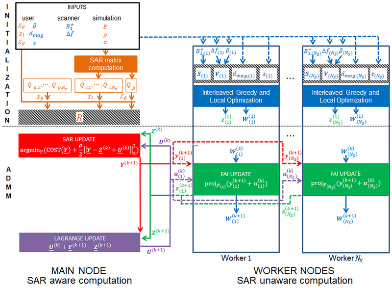
Figure 1:

Flowchart for the IMPULSE optimization algorithm. A main node receives inputs and divides work among N_S worker nodes. The user inputs are χ_p, χ_l, χ_g corresponding to average per channel power, local SAR, and global SAR constraints and β (the slice select subpulse waveform), d_magc (the magnitude of the target excitation map for each slice), and ε (the tolerance on the NRMSE for each slice). Scanner inputs are $B_1^{+}$ the transmit sensitivity maps and Δf the off resonance maps for each channel and each slice. Simulation inputs are E, the electric field over the whole volume for each channel; ρ, the mass density of the tissue model; and σ, the conductivity of the tissue model. The variables in blue which affect the flip angle inhomogeneity of individual slices but not SAR are distributed (indicated by dashed line) to N_S worker nodes corresponding to N_S separate slices to be excited during the scan. During the initialization step, work proceeds on the main node and worker nodes in parallel. On the main node, SAR matrices are formed using the simulation input and these are transformed into the oracle matrix, R, after normalization by the constraints. On the worker nodes, the $B_1^{+}$ maps are flattened to form a matrix S which characterizes the effect of the transmit sensitivity maps on the flip angle, β and Δf are combined into a single matrix V which characterizes the phase accrual from off resonance, and the d_mag and ε values are stored on each worker. In this way the pTx pulse design problem is defined completely by five variables: R which describes cumulative SAR and power information over all slices, and S, V, d_mag, and ε which characterize the flip angle inhomogeneity of each slice. While oracle construction is happening on the main node, SAR unaware interleaved greedy and local optimization occurs on each of the worker nodes for each slice. Spokes are added until the NRMSE tolerance is satisfied. The output is a channel weighting vector z and a matrix W that describes the phase accrual from optimal spokes locations. These variables are initial values for the ADMM algorithm. First a SAR update is performed which serves to reduce the SAR of the pulse while still applying a penalty on the distance from z. The output Y will have lower SAR but could possibly violate the NRMSE tolerance. Then the Y variable is split across slices and distributed to the workers, each of which performs a FAI update where y is projected on to the feasible set to get a vector z that is guaranteed to satisfy the NRMSE tolerance but will have higher SAR. Then the z variables for each slice is sent back to the main node and a composite matrix Z is formed which is used to update the Lagrange multiplier U that serves to enforce consistency between the Y and Z variables. These three updates are performed iteratively until Y ≈ Z at which point the final pulse will have minimum SAR while also satisfying the NRMSE tolerance.