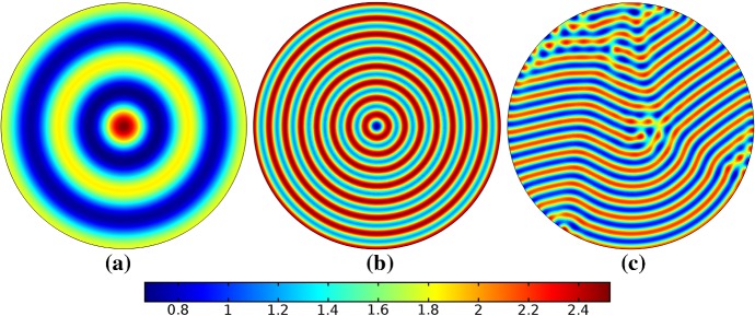
Fig. 16.

Simulations of Eq. (25) with kinetics given by (44) using parameters S2. We plot the distribution of u. a is the pattern at time $T^{\ast }=6\times {10}^4$ on the initial domain, b is the final stationary pattern at the time $T=7.2\times {10}^5$ in this slow growth case, and c is the final pattern for an isotropic growth timescale of $T_g={10}^3$ (Color figure online)